Import Necessary Libraries
![]()
For motivation, watch the following video: https://www.youtube.com/watch?v=aircAruvnKk
To play with a network and visualize what’s happening, check out: https://playground.tensorflow.org/
More visualization and justification of why initialization: https://www.deeplearning.ai/ai-notes/initialization/index.html
A topological explanation and visualization of neural networks: https://colah.github.io/posts/2014-03-NN-Manifolds-Topology/
Import Necessary Libraries
We need to import PyTorch, some submodules like nn for neural networks, optim for optimizers, and DataLoader for efficient data loading.
import torch
import torch.nn as nn
import torch.optim as optim
from torch.utils.data import DataLoader, random_split
from torchvision import datasets, transforms
Load and Preprocess the Dataset
We will load the MNIST dataset using torchvision.datasets, apply transformations such as converting images to tensors, and normalize the pixel values between -1 and 1 using transforms.Normalize.
transform = transforms.Compose([transforms.ToTensor(), transforms.Normalize((0.5,), (0.5,))])

# Download and load the MNIST dataset
mnist_data = datasets.MNIST(root='./data', train=True, download=True, transform=transform)

# Split the dataset into train, dev, and test sets
train_size = int(0.8 * len(mnist_data))  # 80% for training
dev_size = int(0.1 * len(mnist_data))  # 10% for validation (dev)
test_size = len(mnist_data) - train_size - dev_size  # Remaining 10% for testing

train_data, dev_data, test_data = random_split(mnist_data, [train_size, dev_size, test_size])
Use DataLoader for Efficient Data Loading
We will use PyTorch’s DataLoader to load data in batches, which makes training more efficient and allows us to shuffle the training data.
batch_size = 64

# Create DataLoader for train, dev, and test sets
train_loader = DataLoader(train_data, batch_size=batch_size, shuffle=True)
dev_loader = DataLoader(dev_data, batch_size=batch_size, shuffle=False)
test_loader = DataLoader(test_data, batch_size=batch_size, shuffle=False)
Define the Neural Network
We’ll define a simple feedforward neural network with one hidden layer using PyTorch’s nn.Module.
class SimpleNN(nn.Module):
    def __init__(self):
        super(SimpleNN, self).__init__()
        self.fc1 = nn.Linear(28 * 28, 128)  # Input layer (28x28 pixels)
        self.fc2 = nn.Linear(128, 64)  # Hidden layer
        self.fc3 = nn.Linear(64, 10)  # Output layer (10 digits)

    def forward(self, x):
        x = x.view(-1, 28 * 28)  # Flatten the image to a vector of 28x28
        x = torch.relu(self.fc1(x))
        x = torch.relu(self.fc2(x))
        x = self.fc3(x)
        return x
Define Loss and Optimizer
We will use cross-entropy loss for classification and SGD (Stochastic Gradient Descent) as the optimizer.
# Instantiate the model, loss function, and optimizer
model = SimpleNN()
criterion = nn.CrossEntropyLoss()
optimizer = optim.SGD(model.parameters(), lr=0.01)
Train the Network
We will train the model over multiple epochs, performing forward and backward passes, updating weights, and tracking the loss.
# Training loop
epochs = 20

for epoch in range(epochs):
    model.train()  # Set the model to training mode
    running_loss = 0

    for images, labels in train_loader:
        # Zero the parameter gradients
        optimizer.zero_grad()

        # Forward pass
        outputs = model(images)
        loss = criterion(outputs, labels)

        # Backward pass and optimize
        loss.backward()
        optimizer.step()

        running_loss += loss.item()

    # Print loss for the epoch
    print(f'Epoch [{epoch+1}/{epochs}], Loss: {running_loss/len(train_loader):.4f}')
Epoch [1/20], Loss: 1.1366
Epoch [2/20], Loss: 0.4268
Epoch [3/20], Loss: 0.3452
Epoch [4/20], Loss: 0.3106
Epoch [5/20], Loss: 0.2860
Epoch [6/20], Loss: 0.2662
Epoch [7/20], Loss: 0.2497
Epoch [8/20], Loss: 0.2340
Epoch [9/20], Loss: 0.2204
Epoch [10/20], Loss: 0.2072
Epoch [11/20], Loss: 0.1957
Epoch [12/20], Loss: 0.1855
Epoch [13/20], Loss: 0.1754
Epoch [14/20], Loss: 0.1670
Epoch [15/20], Loss: 0.1584
Epoch [16/20], Loss: 0.1504
Epoch [17/20], Loss: 0.1438
Epoch [18/20], Loss: 0.1366
Epoch [19/20], Loss: 0.1306
Epoch [20/20], Loss: 0.1254
Evaluate the Model on the Validation Set
After each epoch, we will evaluate the model on the validation (dev) set to track its accuracy.
import torch.nn.functional as F

def evaluate_model(loader):
    model.eval()  # Set the model to evaluation mode
    total, correct = 0, 0
    with torch.no_grad():  # Disable gradient calculation
        for images, labels in loader:
            outputs = model(images)
            probabilities = F.softmax(outputs, dim=1)
            predicted = torch.argmax(probabilities, dim=1)
            total += labels.size(0)
            correct += (predicted == labels).sum().item()

    return correct / total

# Evaluate on dev set
accuracy = evaluate_model(dev_loader)
print(f'Validation Accuracy: {accuracy * 100:.2f}%')
Validation Accuracy: 95.85%
Test the Model
Finally, after training and validating the model, we evaluate it on the test set to see its generalization performance.
# Evaluate on test set
test_accuracy = evaluate_model(test_loader)
print(f'Test Accuracy: {test_accuracy * 100:.2f}%')
Test Accuracy: 95.37%
import matplotlib.pyplot as plt
import torch.nn.functional as F
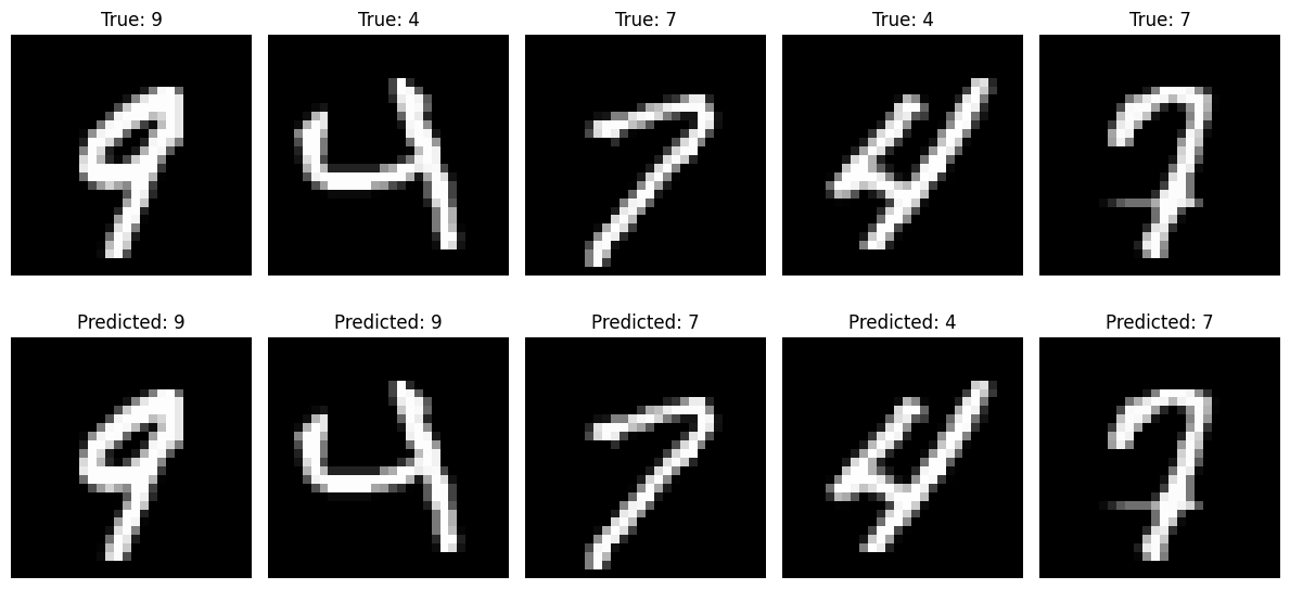
# Function to visualize a few examples before and after training
def visualize_examples(model, data_loader, num_examples=5):
model.eval() # Set the model to evaluation mode
examples_shown = 0
fig, axes = plt.subplots(2, num_examples, figsize=(12, 6)) # 2 rows: before and after training
# Iterate through the data
with torch.no_grad():
for images, labels in data_loader:
# Show the first few examples
if examples_shown >= num_examples:
break
for i in range(len(images)):
if examples_shown >= num_examples:
break
image = images[i].squeeze() # Get the image
label = labels[i].item() # True label
# Predict the label before training
outputs = model(images[i].unsqueeze(0)) # Add batch dimension
probabilities = F.softmax(outputs, dim=1) # Apply softmax
predicted_label = torch.argmax(probabilities, dim=1).item() # Argmax to get predicted class
# Visualize the image
axes[0, examples_shown].imshow(image, cmap='gray')
axes[0, examples_shown].set_title(f"True: {label}")
axes[0, examples_shown].axis('off')
# Visualize the predicted label after training
axes[1, examples_shown].imshow(image, cmap='gray')
axes[1, examples_shown].set_title(f"Predicted: {predicted_label}")
axes[1, examples_shown].axis('off')
examples_shown += 1
plt.tight_layout()
plt.show()
# Visualize 5 examples after training
visualize_examples(model, test_loader, num_examples=5)