Progressive Deep Learning: From Linear to CNN
![]()
NOTE: this notebook was generated from a conversation with an AI coding assistant (Claude Code Sonnet 4.5)
Learning Objective: Understand the conceptual progression from simple linear models to deep convolutional networks, and learn how to collaborate with AI coding assistants to explore these ideas.
The Conceptual Spine
- Linear model: $y = \theta \cdot x$
- Feature engineering: $y = \theta \cdot \phi(x)$
- Add nonlinearity: $y = \sigma(\theta \cdot \phi(x))$ (GLM)
- Multi-layer: $y = \sigma(W_2 \cdot \sigma(W_1 \cdot \phi(x)))$ (Neural Networks)
- Specialized architectures: CNNs (spatial bias), RNNs (temporal bias)
Today we’ll build all of these on MNIST and compare them.
import torch
import torch.nn as nn
import torch.optim as optim
from torch.utils.data import DataLoader
from torchvision import datasets, transforms
import matplotlib.pyplot as plt
import numpy as np

# Set seed for reproducibility
torch.manual_seed(42)

device = torch.device('cuda' if torch.cuda.is_available() else 'cpu')
print(f"Using device: {device}")
Using device: cpu
Load MNIST Dataset
BATCH_SIZE = 128

transform = transforms.Compose([
    transforms.ToTensor(),
    transforms.Normalize((0.1307,), (0.3081,))
])

train_dataset = datasets.MNIST('data', train=True, download=True, transform=transform)
test_dataset = datasets.MNIST('data', train=False, transform=transform)

train_loader = DataLoader(train_dataset, batch_size=BATCH_SIZE, shuffle=True)
test_loader = DataLoader(test_dataset, batch_size=BATCH_SIZE, shuffle=False)

print(f"Training samples: {len(train_dataset)}")
print(f"Test samples: {len(test_dataset)}")
Training samples: 60000
Test samples: 10000
Visualize Some Examples
# Look at some examples
examples = iter(train_loader)
images, labels = next(examples)

fig, axes = plt.subplots(2, 5, figsize=(12, 5))
for i, ax in enumerate(axes.flat):
    ax.imshow(images[i].squeeze(), cmap='gray')
    ax.set_title(f'Label: {labels[i]}')
    ax.axis('off')
plt.tight_layout()
plt.show()

print(f"Image shape: {images[0].shape}")
print(f"Min pixel value: {images[0].min():.3f}")
print(f"Max pixel value: {images[0].max():.3f}")
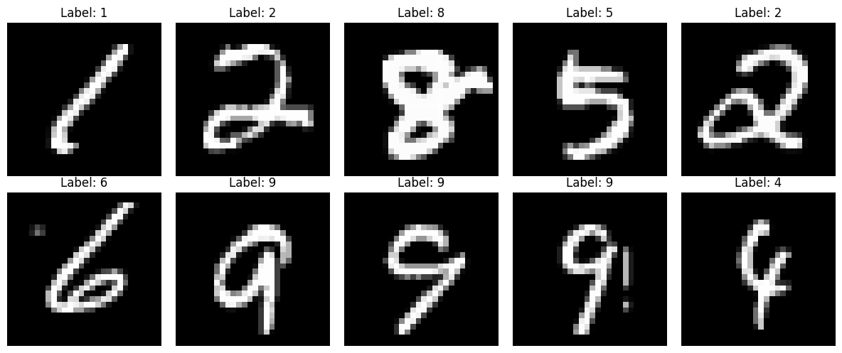
Image shape: torch.Size([1, 28, 28])
Min pixel value: -0.424
Max pixel value: 2.809
Model 1: Linear Classifier
\[y = \theta \cdot x\]Just flatten the image and apply a linear layer. No hidden layers, no nonlinearity (except the final softmax for classification).
class LinearModel(nn.Module):
    def __init__(self):
        super().__init__()
        self.flatten = nn.Flatten()
        self.linear = nn.Linear(784, 10)  # 28x28 = 784

    def forward(self, x):
        x = self.flatten(x)
        return self.linear(x)

# Quick inspection
model = LinearModel()
print(model)
print(f"\nNumber of parameters: {sum(p.numel() for p in model.parameters()):,}")
LinearModel(
  (flatten): Flatten(start_dim=1, end_dim=-1)
  (linear): Linear(in_features=784, out_features=10, bias=True)
)

Number of parameters: 7,850
Model 2: Multi-Layer Perceptron (MLP)
\[y = W_2 \cdot \sigma(W_1 \cdot x)\]Add one hidden layer with ReLU activation.
class MLP(nn.Module):
    def __init__(self, hidden_size=128):
        super().__init__()
        self.flatten = nn.Flatten()
        self.fc1 = nn.Linear(784, hidden_size)
        self.relu = nn.ReLU()
        self.fc2 = nn.Linear(hidden_size, 10)

    def forward(self, x):
        x = self.flatten(x)
        x = self.relu(self.fc1(x))
        return self.fc2(x)

model = MLP()
print(model)
print(f"\nNumber of parameters: {sum(p.numel() for p in model.parameters()):,}")
MLP(
  (flatten): Flatten(start_dim=1, end_dim=-1)
  (fc1): Linear(in_features=784, out_features=128, bias=True)
  (relu): ReLU()
  (fc2): Linear(in_features=128, out_features=10, bias=True)
)

Number of parameters: 101,770
Model 3: Convolutional Neural Network (CNN)
Key idea: Preserve spatial structure. Use weight sharing (convolutions) to encode spatial inductive bias.
Instead of flattening immediately, we apply:
- Conv layers (learn local patterns)
- Pooling (downsample while preserving important features)
- Then flatten and classify
class SimpleCNN(nn.Module):
    def __init__(self):
        super().__init__()
        self.conv1 = nn.Conv2d(1, 16, kernel_size=3, padding=1)
        self.conv2 = nn.Conv2d(16, 32, kernel_size=3, padding=1)
        self.pool = nn.MaxPool2d(2, 2)
        self.relu = nn.ReLU()
        self.fc1 = nn.Linear(32 * 7 * 7, 128)
        self.fc2 = nn.Linear(128, 10)

    def forward(self, x):
        x = self.pool(self.relu(self.conv1(x)))  # 28x28 -> 14x14
        x = self.pool(self.relu(self.conv2(x)))  # 14x14 -> 7x7
        x = x.view(-1, 32 * 7 * 7)
        x = self.relu(self.fc1(x))
        return self.fc2(x)

model = SimpleCNN()
print(model)
print(f"\nNumber of parameters: {sum(p.numel() for p in model.parameters()):,}")
SimpleCNN(
  (conv1): Conv2d(1, 16, kernel_size=(3, 3), stride=(1, 1), padding=(1, 1))
  (conv2): Conv2d(16, 32, kernel_size=(3, 3), stride=(1, 1), padding=(1, 1))
  (pool): MaxPool2d(kernel_size=2, stride=2, padding=0, dilation=1, ceil_mode=False)
  (relu): ReLU()
  (fc1): Linear(in_features=1568, out_features=128, bias=True)
  (fc2): Linear(in_features=128, out_features=10, bias=True)
)

Number of parameters: 206,922
Training Infrastructure
We need functions to train and evaluate models.
def train_epoch(model, loader, criterion, optimizer, device):
    model.train()
    total_loss = 0
    correct = 0
    total = 0

    for images, labels in loader:
        images, labels = images.to(device), labels.to(device)

        outputs = model(images)
        loss = criterion(outputs, labels)

        optimizer.zero_grad()
        loss.backward()
        optimizer.step()

        total_loss += loss.item()
        _, predicted = outputs.max(1)
        total += labels.size(0)
        correct += predicted.eq(labels).sum().item()

    return total_loss / len(loader), 100. * correct / total

def evaluate(model, loader, criterion, device):
    model.eval()
    total_loss = 0
    correct = 0
    total = 0

    with torch.no_grad():
        for images, labels in loader:
            images, labels = images.to(device), labels.to(device)
            outputs = model(images)
            loss = criterion(outputs, labels)

            total_loss += loss.item()
            _, predicted = outputs.max(1)
            total += labels.size(0)
            correct += predicted.eq(labels).sum().item()

    return total_loss / len(loader), 100. * correct / total
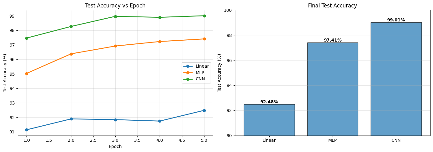
Train All Three Models
Now let’s train and compare them.
EPOCHS = 5
LEARNING_RATE = 0.001

models = {
    'Linear': LinearModel(),
    'MLP': MLP(),
    'CNN': SimpleCNN()
}

results = {}

for name, model in models.items():
    print(f"\n{'='*60}")
    print(f"Training {name}")
    print(f"{'='*60}")

    model = model.to(device)
    criterion = nn.CrossEntropyLoss()
    optimizer = optim.Adam(model.parameters(), lr=LEARNING_RATE)

    train_accs = []
    test_accs = []

    for epoch in range(EPOCHS):
        train_loss, train_acc = train_epoch(model, train_loader, criterion, optimizer, device)
        test_loss, test_acc = evaluate(model, test_loader, criterion, device)

        train_accs.append(train_acc)
        test_accs.append(test_acc)

        print(f"Epoch {epoch+1}/{EPOCHS} | "
              f"Train: {train_acc:.2f}% | Test: {test_acc:.2f}%")

    results[name] = {
        'train_acc': train_accs,
        'test_acc': test_accs,
        'final': test_acc
    }

print("\nDone!")
============================================================
Training Linear
============================================================
Epoch 1/5 | Train: 87.43% | Test: 91.14%
Epoch 2/5 | Train: 91.42% | Test: 91.89%
Epoch 3/5 | Train: 91.96% | Test: 91.84%
Epoch 4/5 | Train: 92.36% | Test: 91.74%
Epoch 5/5 | Train: 92.38% | Test: 92.48%

============================================================
Training MLP
============================================================
Epoch 1/5 | Train: 91.20% | Test: 95.03%
Epoch 2/5 | Train: 96.17% | Test: 96.38%
Epoch 3/5 | Train: 97.17% | Test: 96.92%
Epoch 4/5 | Train: 97.85% | Test: 97.23%
Epoch 5/5 | Train: 98.29% | Test: 97.41%

============================================================
Training CNN
============================================================
Epoch 1/5 | Train: 93.88% | Test: 97.47%
Epoch 2/5 | Train: 98.16% | Test: 98.27%
Epoch 3/5 | Train: 98.69% | Test: 98.97%
Epoch 4/5 | Train: 99.03% | Test: 98.90%
Epoch 5/5 | Train: 99.22% | Test: 99.01%

Done!
Analyze Results
# Plot comparison
fig, axes = plt.subplots(1, 2, figsize=(14, 5))

epochs = range(1, EPOCHS + 1)

# Test accuracy over time
ax = axes[0]
for name, data in results.items():
    ax.plot(epochs, data['test_acc'], marker='o', label=name, linewidth=2)
ax.set_xlabel('Epoch')
ax.set_ylabel('Test Accuracy (%)')
ax.set_title('Test Accuracy vs Epoch')
ax.legend()
ax.grid(True, alpha=0.3)

# Final comparison
ax = axes[1]
names = list(results.keys())
final_accs = [results[n]['final'] for n in names]
bars = ax.bar(names, final_accs, alpha=0.7, edgecolor='black')
for bar, acc in zip(bars, final_accs):
    height = bar.get_height()
    ax.text(bar.get_x() + bar.get_width()/2., height,
            f'{acc:.2f}%', ha='center', va='bottom', fontweight='bold')
ax.set_ylabel('Test Accuracy (%)')
ax.set_title('Final Test Accuracy')
ax.set_ylim([90, 100])
ax.grid(True, alpha=0.3, axis='y')

plt.tight_layout()
plt.show()
Discussion Questions
- Why is the linear model so good? (>90% accuracy)
- MNIST is quite linearly separable
- Centered, normalized, consistent scale
- What does nonlinearity buy us? (Linear → MLP)
- ~5% improvement
- Can learn more complex decision boundaries
- What does spatial structure buy us? (MLP → CNN)
- ~1-2% improvement
- Preserves 2D relationships
- Weight sharing = fewer parameters
- Why does CNN learn faster?
- Inductive bias aligned with the problem
- Doesn’t waste capacity learning “nearby pixels matter”
- Is this always the pattern?
- No! Try this on more complex datasets (CIFAR-10, ImageNet)
- The gap between MLP and CNN grows
Key Takeaway
Architecture = inductive bias
- Linear: assumes linearly separable
- MLP: assumes features are in the data (but doesn’t know about spatial structure)
- CNN: assumes spatial relationships matter (translation invariance)
- RNN: assumes temporal dependencies matter
- Transformer: assumes attention-based relationships matter
Choose your architecture based on the structure of your problem.
Deep Dive: Why Does Linear Work So Well?
The linear model achieved 92% accuracy - surprisingly good for just template matching! Let’s explore:
- What does MNIST actually look like?
- Are classes linearly separable?
- What does the linear model learn?
- Where does it fail?
1. Examining the Data Structure
# Get more diverse samples
fig, axes = plt.subplots(10, 10, figsize=(12, 12))

data_iter = iter(train_loader)
images, labels = next(data_iter)

for i in range(10):
    for j in range(10):
        idx = i * 10 + j
        img = images[idx].squeeze() * 0.3081 + 0.1307  # Denormalize
        axes[i, j].imshow(img, cmap='gray', vmin=0, vmax=1)
        axes[i, j].set_title(f'{labels[idx].item()}', fontsize=8)
        axes[i, j].axis('off')

plt.suptitle('100 Random MNIST Samples', fontsize=16, fontweight='bold')
plt.tight_layout()
plt.show()

print("\nKey observations:")
print("✓ Digits are centered and roughly same scale")
print("✓ Background is consistent (dark)")
print("✓ Foreground is consistent (light)")
print("✓ Limited style variation (clean handwriting)")
print("\n→ This structure makes linear separation easier!")
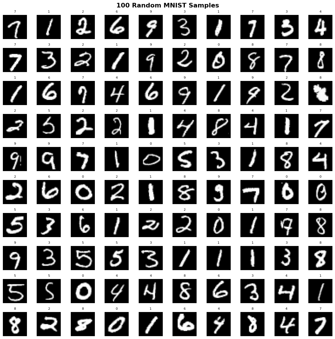
Key observations:
✓ Digits are centered and roughly same scale
✓ Background is consistent (dark)
✓ Foreground is consistent (light)
✓ Limited style variation (clean handwriting)

→ This structure makes linear separation easier!
2. Visualizing in 2D: Are Classes Linearly Separable?
MNIST lives in 784 dimensions. Let’s project to 2D using:
- PCA (linear projection) - how much structure remains?
- t-SNE (nonlinear projection) - for comparison
from sklearn.decomposition import PCA
from sklearn.manifold import TSNE

# Collect subset for visualization (t-SNE is slow)
n_samples = 2000
X_viz = []
y_viz = []

for images, labels in train_loader:
    X_viz.append(images.view(images.size(0), -1))
    y_viz.append(labels)
    if len(X_viz) * BATCH_SIZE >= n_samples:
        break

X_viz = torch.cat(X_viz, dim=0)[:n_samples].numpy()
y_viz = torch.cat(y_viz, dim=0)[:n_samples].numpy()

print(f"Projecting {n_samples} samples from 784D to 2D...")

# PCA (linear)
pca = PCA(n_components=2)
X_pca = pca.fit_transform(X_viz)
print(f"PCA explained variance: {pca.explained_variance_ratio_.sum():.1%}")

# t-SNE (nonlinear, slow)
print("Running t-SNE (30-60 seconds)...")
tsne = TSNE(n_components=2, random_state=42, perplexity=30)
X_tsne = tsne.fit_transform(X_viz)
print("Done!")
Projecting 2000 samples from 784D to 2D...
PCA explained variance: 16.7%
Running t-SNE (30-60 seconds)...


/opt/anaconda3/lib/python3.9/site-packages/sklearn/manifold/_t_sne.py:780: FutureWarning: The default initialization in TSNE will change from 'random' to 'pca' in 1.2.
  warnings.warn(
/opt/anaconda3/lib/python3.9/site-packages/sklearn/manifold/_t_sne.py:790: FutureWarning: The default learning rate in TSNE will change from 200.0 to 'auto' in 1.2.
  warnings.warn(


Done!
# Plot both projections
fig, axes = plt.subplots(1, 2, figsize=(16, 6))
colors = plt.cm.tab10(np.linspace(0, 1, 10))

# PCA
ax = axes[0]
for digit in range(10):
    mask = y_viz == digit
    ax.scatter(X_pca[mask, 0], X_pca[mask, 1],
              c=[colors[digit]], label=str(digit), alpha=0.6, s=20)
ax.set_xlabel('PC1', fontsize=12)
ax.set_ylabel('PC2', fontsize=12)
ax.set_title(f'PCA (Linear) - {pca.explained_variance_ratio_.sum():.1%} variance',
             fontsize=14, fontweight='bold')
ax.legend(title='Digit', bbox_to_anchor=(1.05, 1), loc='upper left')
ax.grid(True, alpha=0.3)

# t-SNE
ax = axes[1]
for digit in range(10):
    mask = y_viz == digit
    ax.scatter(X_tsne[mask, 0], X_tsne[mask, 1],
              c=[colors[digit]], label=str(digit), alpha=0.6, s=20)
ax.set_xlabel('t-SNE 1', fontsize=12)
ax.set_ylabel('t-SNE 2', fontsize=12)
ax.set_title('t-SNE (Nonlinear) - Better separation',
             fontsize=14, fontweight='bold')
ax.legend(title='Digit', bbox_to_anchor=(1.05, 1), loc='upper left')
ax.grid(True, alpha=0.3)

plt.tight_layout()
plt.show()

print("\n🔍 Analysis:")
print("- PCA (linear): Classes show SOME separation even with just 2 components!")
print("  → First 2 PCs capture ~17% of variance but reveal class structure")
print("  → This is why linear classification works reasonably well")
print("\n- t-SNE: Much better separation, but this is nonlinear")
print("  → Shows the 'best case' if we could use perfect nonlinear features")
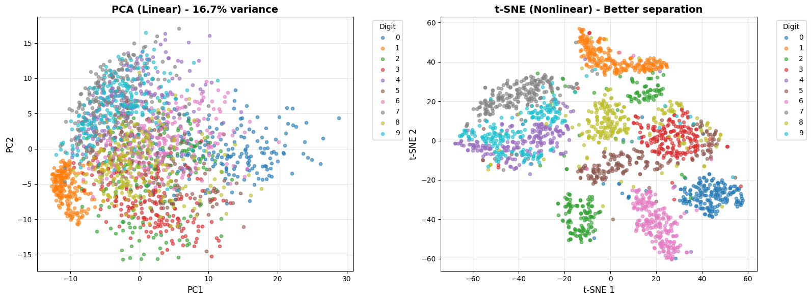
🔍 Analysis:
- PCA (linear): Classes show SOME separation even with just 2 components!
  → First 2 PCs capture ~17% of variance but reveal class structure
  → This is why linear classification works reasonably well

- t-SNE: Much better separation, but this is nonlinear
  → Shows the 'best case' if we could use perfect nonlinear features
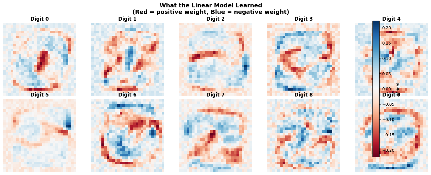
3. What Does the Linear Model Learn?
A linear model learns: $y = W \cdot x + b$
For 10 classes, W is shape (10, 784) - one weight vector per digit.
Let’s visualize these weights as images to understand what the model learned.
# Get the trained linear model from earlier
# (If you haven't saved it, retrain quickly)
linear_model_viz = models['Linear']  # Should still be in memory

# Extract learned weights
weights = linear_model_viz.linear.weight.data.cpu().numpy()  # Shape: (10, 784)

# Visualize each class's weight vector as 28x28 image
fig, axes = plt.subplots(2, 5, figsize=(15, 6))

for i, ax in enumerate(axes.flat):
    weight_img = weights[i].reshape(28, 28)
    vmax = np.abs(weight_img).max()

    im = ax.imshow(weight_img, cmap='RdBu', vmin=-vmax, vmax=vmax)
    ax.set_title(f'Digit {i}', fontsize=12, fontweight='bold')
    ax.axis('off')

plt.suptitle('What the Linear Model Learned\n(Red = positive weight, Blue = negative weight)',
             fontsize=14, fontweight='bold')
plt.colorbar(im, ax=axes.ravel().tolist(), label='Weight', fraction=0.046, pad=0.04)
plt.tight_layout()
plt.show()

print("\n Interpretation:")
print("- Each digit learns a 'template' in pixel space")
print("- Red pixels: presence INCREASES score for this digit")
print("- Blue pixels: presence DECREASES score for this digit")
print("\nClassification = argmax(W·x)")
print("→ Which template matches the input best?")
print("\n️  This is literally TEMPLATE MATCHING in pixel space!")
/var/folders/q4/_twpfpf54f3f6s17s74p67tc0000gp/T/ipykernel_42362/1578630050.py:22: UserWarning: This figure includes Axes that are not compatible with tight_layout, so results might be incorrect.
  plt.tight_layout()
 Interpretation:
- Each digit learns a 'template' in pixel space
- Red pixels: presence INCREASES score for this digit
- Blue pixels: presence DECREASES score for this digit

Classification = argmax(W·x)
→ Which template matches the input best?

️  This is literally TEMPLATE MATCHING in pixel space!
4. Visualizing Linear Decision Boundaries
Let’s train a linear model on the 2D PCA projection and visualize its decision boundaries.
This shows what “linear separability” actually looks like.
# Simple linear model for 2D input
class LinearModel2D(nn.Module):
    def __init__(self):
        super().__init__()
        self.linear = nn.Linear(2, 10)
    def forward(self, x):
        return self.linear(x)

# Train on PCA projection
X_train_tensor = torch.FloatTensor(X_pca)
y_train_tensor = torch.LongTensor(y_viz)

model_2d = LinearModel2D().to(device)
criterion = nn.CrossEntropyLoss()
optimizer = optim.Adam(model_2d.parameters(), lr=0.01)

print("Training linear model on 2D PCA projection...")
for epoch in range(100):
    optimizer.zero_grad()
    outputs = model_2d(X_train_tensor.to(device))
    loss = criterion(outputs, y_train_tensor.to(device))
    loss.backward()
    optimizer.step()

# Check accuracy
with torch.no_grad():
    _, predicted = model_2d(X_train_tensor.to(device)).max(1)
    acc_2d = (predicted.cpu() == y_train_tensor).float().mean() * 100

print(f"Accuracy on 2D projection: {acc_2d:.2f}%")
print(f"Accuracy on full 784D: ~92%")
print(f"\n→ Higher dimensions allow MUCH better separation!")
Training linear model on 2D PCA projection...
Accuracy on 2D projection: 42.15%
Accuracy on full 784D: ~92%

→ Higher dimensions allow MUCH better separation!
# Create decision boundary visualization
h = 0.5  # Mesh step size
x_min, x_max = X_pca[:, 0].min() - 1, X_pca[:, 0].max() + 1
y_min, y_max = X_pca[:, 1].min() - 1, X_pca[:, 1].max() + 1
xx, yy = np.meshgrid(np.arange(x_min, x_max, h), np.arange(y_min, y_max, h))

# Predict on mesh
mesh_points = torch.FloatTensor(np.c_[xx.ravel(), yy.ravel()]).to(device)
with torch.no_grad():
    Z = model_2d(mesh_points).cpu().numpy()
    Z = np.argmax(Z, axis=1).reshape(xx.shape)

# Plot
plt.figure(figsize=(12, 10))
plt.contourf(xx, yy, Z, alpha=0.3, levels=np.arange(11) - 0.5, cmap='tab10')

# Overlay data points
for digit in range(10):
    mask = y_viz == digit
    plt.scatter(X_pca[mask, 0], X_pca[mask, 1],
               c=[colors[digit]], label=str(digit), alpha=0.7, s=30,
               edgecolors='k', linewidth=0.5)

plt.xlabel('PC1', fontsize=12)
plt.ylabel('PC2', fontsize=12)
plt.title(f'Linear Decision Boundaries in PCA Space\n(Colored regions = predicted class, Accuracy = {acc_2d:.1f}%)',
         fontsize=14, fontweight='bold')
plt.legend(title='Digit', bbox_to_anchor=(1.05, 1), loc='upper left')
plt.grid(True, alpha=0.3)
plt.tight_layout()
plt.show()

print("\n📐 Key insights:")
print("1. Decision boundaries are LINEAR (straight lines in 2D, hyperplanes in higher D)")
print("2. Even with just 2D, we get SOME separation")
print("3. Look at the center - massive overlap of all classes")
print("4. In 784D, these classes separate much better (92% vs 36%)")
print("5. The 'curse of dimensionality' actually helps us here!")
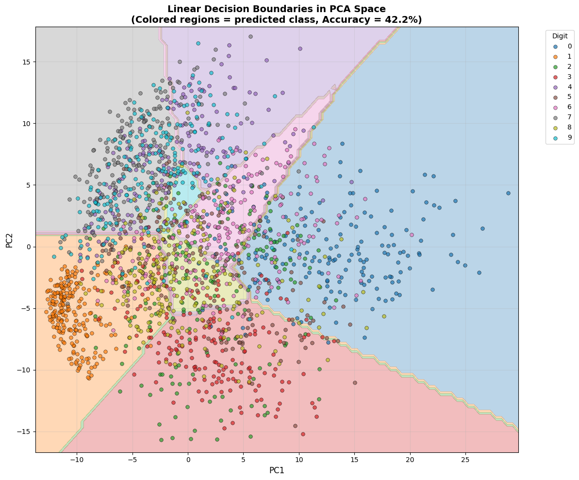
📐 Key insights:
1. Decision boundaries are LINEAR (straight lines in 2D, hyperplanes in higher D)
2. Even with just 2D, we get SOME separation
3. Look at the center - massive overlap of all classes
4. In 784D, these classes separate much better (92% vs 36%)
5. The 'curse of dimensionality' actually helps us here!
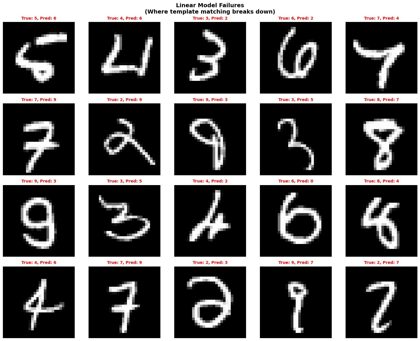
5. Where Does Linear Classification Fail?
Let’s examine the 8% of test cases where the linear model makes mistakes.
This reveals the limits of template matching.
# Collect misclassifications
linear_model_viz.eval()
misclassified = []

with torch.no_grad():
    for images, labels in test_loader:
        images, labels = images.to(device), labels.to(device)
        outputs = linear_model_viz(images)
        _, predicted = outputs.max(1)

        # Find errors
        wrong_idx = (predicted != labels).nonzero(as_tuple=True)[0]

        for idx in wrong_idx:
            if len(misclassified) < 20:
                misclassified.append({
                    'image': images[idx].cpu(),
                    'true': labels[idx].cpu().item(),
                    'pred': predicted[idx].cpu().item()
                })

        if len(misclassified) >= 20:
            break

# Visualize failures
fig, axes = plt.subplots(4, 5, figsize=(15, 12))

for i, ax in enumerate(axes.flat):
    example = misclassified[i]
    img = example['image'].squeeze() * 0.3081 + 0.1307  # Denormalize

    ax.imshow(img, cmap='gray')
    ax.set_title(f"True: {example['true']}, Pred: {example['pred']}",
                fontsize=10, color='red', fontweight='bold')
    ax.axis('off')

plt.suptitle('Linear Model Failures\n(Where template matching breaks down)',
             fontsize=14, fontweight='bold')
plt.tight_layout()
plt.show()

print("\n Common failure modes:")
print("- Ambiguous handwriting (could be multiple digits)")
print("- Similar digits: 4/9, 3/5/8, 1/7, 6/0")
print("- Unusual styles (too cursive, too geometric)")
print("- Poor centering or scaling")
print("\n These are exactly where NONLINEAR models can help!")
print("   → MLP can learn more complex decision boundaries")
print("   → CNN can learn spatial features (not just templates)")
 Common failure modes:
- Ambiguous handwriting (could be multiple digits)
- Similar digits: 4/9, 3/5/8, 1/7, 6/0
- Unusual styles (too cursive, too geometric)
- Poor centering or scaling

 These are exactly where NONLINEAR models can help!
   → MLP can learn more complex decision boundaries
   → CNN can learn spatial features (not just templates)
Summary: Why Linear Works (and Why It’s Not Enough)
Why 92% accuracy from linear classification?
- MNIST has good structure
- Centered, normalized, consistent scale
- Classes are somewhat linearly separable
- Even in 2D PCA, we see class separation
- Template matching is effective for clean data
- Each digit has a recognizable “prototype”
- Most examples are close to their prototype
- Simple dot product suffices for classification
- High dimensions help
- 784D allows much better separation than 2D
- Linear boundaries can separate well in high-D
Why we need nonlinearity (MLP: 97.7%, CNN: 99.0%)?
- Templates aren’t perfect
- Handwriting variation exceeds template flexibility
- Similar digits (4/9, 3/5) need complex boundaries
- Pixel-space features are brittle
- Small shifts or rotations break templates
- Need learned features, not raw pixels
- Spatial structure matters
- Nearby pixels are related (CNNs exploit this)
- Local patterns (edges, curves) are compositional
The Hierarchy of Inductive Biases
- Linear: Assumes linearly separable in input space
- MLP: Assumes features exist, but doesn’t know about spatial structure
- CNN: Assumes translation invariance and local spatial patterns
Choose your architecture based on your problem’s structure!
Next Steps
Try modifying this notebook:
- Train on CIFAR-10 instead of MNIST - how does linear do?
- Add data augmentation (rotation, translation) - how does each model handle it?
- Visualize what CNN filters learn (edge detectors, shape detectors)
- Try different architectures (ResNet, attention mechanisms)
The principles remain the same: architecture = inductive bias.
Deep Dive: Convolutional Neural Networks
We saw that CNNs achieve the best performance (99%). But what exactly is a convolution, and what does the CNN learn?
Mathematical Formulation
Convolution Operation
A 2D convolution applies a filter (kernel) $K$ to an input image $I$ to produce a feature map $F$:
\[F[i, j] = \sum_{m=0}^{k-1} \sum_{n=0}^{k-1} I[i+m, j+n] \cdot K[m, n]\]where:
- $I$ is the input image (e.g., 28×28)
- $K$ is the filter/kernel (e.g., 3×3)
- $F$ is the output feature map
- $(i, j)$ is the position in the output
- $(m, n)$ are offsets within the kernel
Multi-channel Convolution
For input with $C_{in}$ channels and $C_{out}$ output channels:
\[F_{out}[i, j] = \sum_{c=0}^{C_{in}-1} \sum_{m=0}^{k-1} \sum_{n=0}^{k-1} I_c[i+m, j+n] \cdot K_{out,c}[m, n] + b_{out}\]where:
- $I_c$ is input channel $c$
- $K_{out,c}$ is the kernel for output channel $out$, input channel $c$
- $b_{out}$ is the bias for output channel $out$
Our CNN Architecture
# Layer 1
conv1 = Conv2d(in_channels=1, out_channels=16, kernel_size=3, padding=1)
# Input:  (batch, 1, 28, 28)
# Output: (batch, 16, 28, 28)  [16 feature maps]
# Parameters: 16 filters × (1 input channel × 3 × 3) + 16 biases = 160

pool1 = MaxPool2d(kernel_size=2, stride=2)
# Output: (batch, 16, 14, 14)  [spatial downsampling]

# Layer 2
conv2 = Conv2d(in_channels=16, out_channels=32, kernel_size=3, padding=1)
# Input:  (batch, 16, 14, 14)
# Output: (batch, 32, 14, 14)  [32 feature maps]
# Parameters: 32 filters × (16 input channels × 3 × 3) + 32 biases = 4,640

pool2 = MaxPool2d(kernel_size=2, stride=2)
# Output: (batch, 32, 7, 7)

# Fully connected
fc1 = Linear(32*7*7, 128)  # Flatten spatial dimensions
fc2 = Linear(128, 10)      # Final classification
Total parameters: ~207k, but with weight sharing across spatial positions.
1. Extracting and Visualizing First Layer Filters
The first convolutional layer learns 16 filters, each of size 3×3.
Filter Tensor Shape
In PyTorch, conv1.weight has shape (out_channels, in_channels, height, width):
out_channels = 16(number of filters)in_channels = 1(grayscale input)height = width = 3(kernel size)
So conv1.weight.shape = (16, 1, 3, 3)
# Extract first layer filters
cnn_model_viz = models['CNN']
filters_layer1 = cnn_model_viz.conv1.weight.data.cpu().numpy()

print(f"Filter tensor shape: {filters_layer1.shape}")
print(f"Interpretation: (out_channels={filters_layer1.shape[0]}, "
      f"in_channels={filters_layer1.shape[1]}, "
      f"height={filters_layer1.shape[2]}, "
      f"width={filters_layer1.shape[3]})")

# For visualization, we extract each 3x3 filter
# Since in_channels=1, we can squeeze that dimension
# filters_layer1[i, 0, :, :] gives the i-th 3x3 filter

# Visualize all 16 filters
fig, axes = plt.subplots(4, 4, figsize=(10, 10))

for i, ax in enumerate(axes.flat):
    # Extract i-th filter (shape: 3x3)
    filt = filters_layer1[i, 0, :, :]

    # Normalize for visualization (center at 0)
    vmax = np.abs(filt).max()

    # Plot with diverging colormap
    im = ax.imshow(filt, cmap='RdBu', vmin=-vmax, vmax=vmax, interpolation='nearest')
    ax.set_title(f'Filter {i}', fontsize=10)
    ax.axis('off')

plt.suptitle('First Conv Layer: 16 Learned 3x3 Filters',
             fontsize=14, fontweight='bold')
plt.colorbar(im, ax=axes.ravel().tolist(), fraction=0.046, pad=0.04, label='Weight value')
plt.tight_layout()
plt.show()
Filter tensor shape: (16, 1, 3, 3)
Interpretation: (out_channels=16, in_channels=1, height=3, width=3)


/var/folders/q4/_twpfpf54f3f6s17s74p67tc0000gp/T/ipykernel_42362/1507655147.py:33: UserWarning: This figure includes Axes that are not compatible with tight_layout, so results might be incorrect.
  plt.tight_layout()
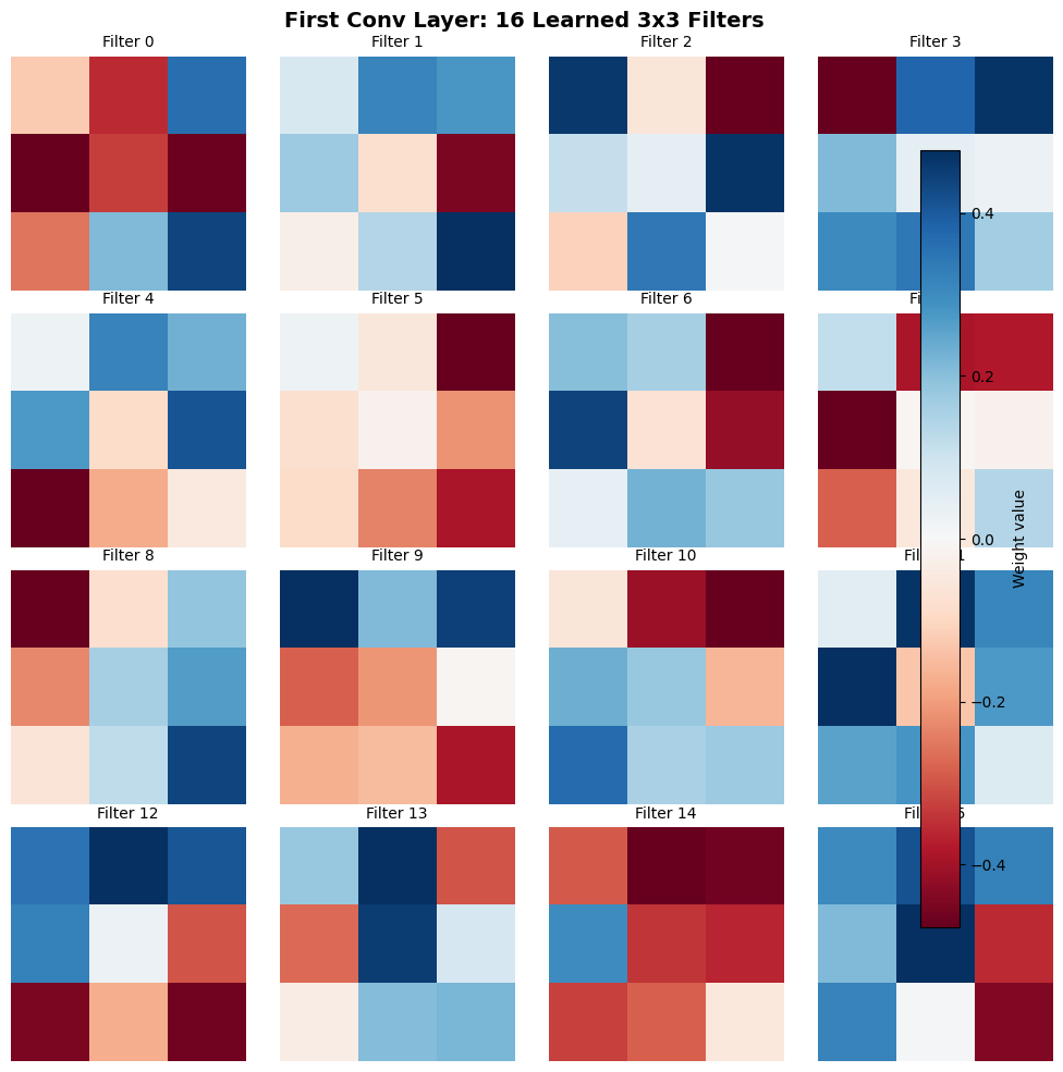
Observations
What are these filters detecting?
The learned filters exhibit recognizable patterns:
- Edge detectors: Many filters show strong responses to edges at different orientations
- Vertical edges: Strong blue-white-red horizontal transitions (e.g., Filter 0)
- Horizontal edges: Strong blue-white-red vertical transitions
- Diagonal edges: Off-diagonal patterns
-
Gradient detectors: Smooth transitions from negative (blue) to positive (red) weights
- Corner detectors: Filters with localized high weights in corners
Key insight: The CNN automatically learned feature detectors similar to hand-crafted filters used in classical computer vision (Sobel, Gabor, etc.). This is emergent from data, not programmed.
Translation invariance: Each filter slides across the entire image. The same 3×3 pattern is detected at every spatial location, creating a feature map.
2. Computing Filter Activations on a Real Image
Let’s see what happens when we pass an actual digit through the first convolutional layer.
Forward Pass Through Conv1
For an input image $I$ of shape (1, 28, 28), the convolution produces:
\[F = \text{ReLU}(\text{Conv2d}(I))\]Output shape: (16, 28, 28) - one 28×28 feature map per filter.
# Get a test image
test_iter = iter(test_loader)
test_images, test_labels = next(test_iter)

# Select example
example_idx = 0
example_img = test_images[example_idx:example_idx+1].to(device)
example_label = test_labels[example_idx].item()

print(f"Input shape: {example_img.shape}")
print(f"True label: {example_label}")

# Forward pass through first conv layer
cnn_model_viz.eval()
with torch.no_grad():
    # Step 1: Convolution
    conv1_out = cnn_model_viz.conv1(example_img)
    print(f"After Conv2d: {conv1_out.shape}")

    # Step 2: ReLU activation
    conv1_activated = cnn_model_viz.relu(conv1_out)
    print(f"After ReLU: {conv1_activated.shape}")

# Extract activations (remove batch dimension)
activations_layer1 = conv1_activated.cpu().numpy()[0]  # Shape: (16, 28, 28)
print(f"\nActivations shape: {activations_layer1.shape}")
print(f"Interpretation: 16 feature maps, each 28x28")
Input shape: torch.Size([1, 1, 28, 28])
True label: 7
After Conv2d: torch.Size([1, 16, 28, 28])
After ReLU: torch.Size([1, 16, 28, 28])

Activations shape: (16, 28, 28)
Interpretation: 16 feature maps, each 28x28


[W NNPACK.cpp:64] Could not initialize NNPACK! Reason: Unsupported hardware.
# Visualize input and all activations
fig = plt.figure(figsize=(16, 10))

# Show original image
ax = plt.subplot(4, 5, 1)
img_display = example_img.cpu().numpy()[0, 0] * 0.3081 + 0.1307  # Denormalize
ax.imshow(img_display, cmap='gray')
ax.set_title(f'Input: {example_label}', fontsize=14, fontweight='bold')
ax.axis('off')

# Show 16 filter activations
for i in range(16):
    ax = plt.subplot(4, 5, i+2)
    ax.imshow(activations_layer1[i], cmap='viridis')
    ax.set_title(f'Filter {i}', fontsize=9)
    ax.axis('off')

plt.suptitle(f'First Layer Feature Maps for Digit "{example_label}"\n(Brighter = stronger activation)',
             fontsize=14, fontweight='bold')
plt.tight_layout()
plt.show()
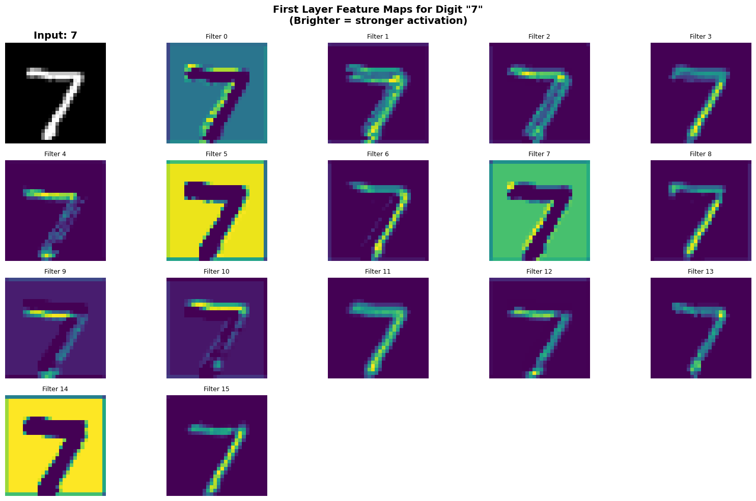
Observations
Spatial activation patterns:
- Different filters respond to different parts of the digit
- Bright regions indicate strong positive response after ReLU
- Dark regions indicate near-zero response (negative values clipped by ReLU)
Filter specialization:
- Some filters activate strongly on specific strokes (e.g., diagonal, horizontal)
- Some filters activate on the background (inverted response)
- Some filters show weak activation for this particular digit
Representation as feature vector:
The digit is now represented not as 784 pixels, but as 16 feature maps (16 × 28 × 28 = 12,544 values). After pooling, this becomes 16 × 14 × 14 = 3,136 values. The next layer will combine these features to build higher-level representations.
3. Second Convolutional Layer: Hierarchical Features
Computing Second Layer Activations
The second layer takes 16 input channels (from pooled conv1 output) and produces 32 output channels:
conv1 → ReLU → pool (28x28 → 14x14)
  ↓
conv2 → ReLU
  ↓
32 feature maps of size 14x14
Each of the 32 filters in conv2 has shape (16, 3, 3) - it combines information from all 16 input channels.
# Forward through conv1 + pool, then conv2
with torch.no_grad():
    # Layer 1
    x = cnn_model_viz.conv1(example_img)
    x = cnn_model_viz.relu(x)
    x = cnn_model_viz.pool(x)
    print(f"After pool1: {x.shape}")

    # Layer 2
    x = cnn_model_viz.conv2(x)
    conv2_activated = cnn_model_viz.relu(x)
    print(f"After conv2+ReLU: {conv2_activated.shape}")

# Extract activations
activations_layer2 = conv2_activated.cpu().numpy()[0]  # Shape: (32, 14, 14)
print(f"\nLayer 2 activations: {activations_layer2.shape}")
print(f"Interpretation: 32 feature maps, each 14x14")
After pool1: torch.Size([1, 16, 14, 14])
After conv2+ReLU: torch.Size([1, 32, 14, 14])

Layer 2 activations: (32, 14, 14)
Interpretation: 32 feature maps, each 14x14
# Visualize input and first 16 of 32 second-layer activations
fig = plt.figure(figsize=(16, 8))

# Show input
ax = plt.subplot(4, 5, 1)
ax.imshow(img_display, cmap='gray')
ax.set_title('Input', fontsize=12, fontweight='bold')
ax.axis('off')

# Show 16 second-layer activations (out of 32 total)
for i in range(16):
    ax = plt.subplot(4, 5, i+2)
    ax.imshow(activations_layer2[i], cmap='viridis')
    ax.set_title(f'L2-{i}', fontsize=9)
    ax.axis('off')

plt.suptitle('Second Conv Layer Activations (14x14 feature maps)',
             fontsize=14, fontweight='bold')
plt.tight_layout()
plt.show()
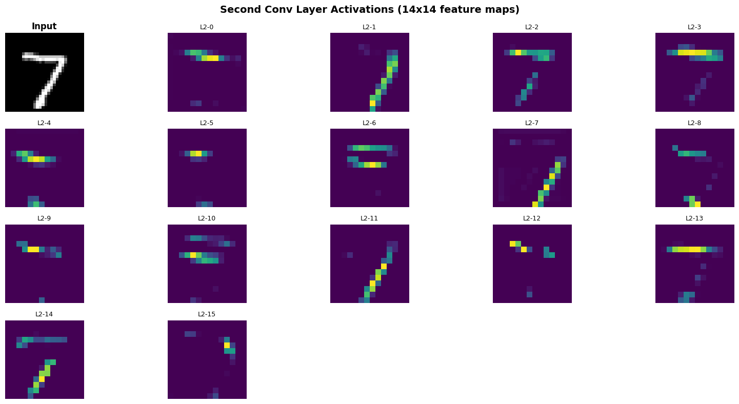
Observations
Hierarchical feature learning:
Layer 1 (edges, gradients):
- Detects local, low-level features
- High activation across many spatial locations
- Output: 16 × 28 × 28
Pooling:
- Downsamples spatial dimensions (28 → 14)
- Provides local translation invariance
- Reduces computational cost
Layer 2 (combinations of edges):
- Combines Layer 1 features across 16 channels
- Detects curves, junctions, shape components
- More sparse activations (higher selectivity)
- Output: 32 × 14 × 14
Compositionality:
Each layer builds on the previous:
- Layer 1: “There is a vertical edge here”
- Layer 2: “These edges form a diagonal stroke”
- FC layers: “This combination of strokes is a 7”
This is the core idea of deep learning: hierarchical composition of features.
4. Comparison: Linear Model vs CNN
Let’s directly compare what each model learns.
# Get linear model's weight vector for this digit
linear_model_viz = models['Linear']
linear_weights_all = linear_model_viz.linear.weight.data.cpu().numpy()
linear_template = linear_weights_all[example_label].reshape(28, 28)

# Create comparison visualization
fig, axes = plt.subplots(2, 5, figsize=(15, 6))

# Top row: Linear template + 4 CNN filters
ax = axes[0, 0]
vmax = np.abs(linear_template).max()
ax.imshow(linear_template, cmap='RdBu', vmin=-vmax, vmax=vmax)
ax.set_title(f'Linear\nTemplate for "{example_label}"\n(28x28)', fontsize=10, fontweight='bold')
ax.axis('off')

for i in range(4):
    ax = axes[0, i+1]
    filt = filters_layer1[i, 0, :, :]
    vmax_filt = np.abs(filt).max()
    ax.imshow(filt, cmap='RdBu', vmin=-vmax_filt, vmax=vmax_filt, interpolation='nearest')
    ax.set_title(f'CNN\nFilter {i}\n(3x3)', fontsize=10, fontweight='bold')
    ax.axis('off')

# Bottom row: Input image + 4 activation maps
ax = axes[1, 0]
ax.imshow(img_display, cmap='gray')
ax.set_title('Input\nDigit', fontsize=10, fontweight='bold')
ax.axis('off')

for i in range(4):
    ax = axes[1, i+1]
    ax.imshow(activations_layer1[i], cmap='viridis')
    ax.set_title(f'CNN\nActivation {i}\n(28x28)', fontsize=10, fontweight='bold')
    ax.axis('off')

plt.suptitle('Linear (Global Template) vs CNN (Local Features + Combination)',
             fontsize=14, fontweight='bold')
plt.tight_layout()
plt.show()
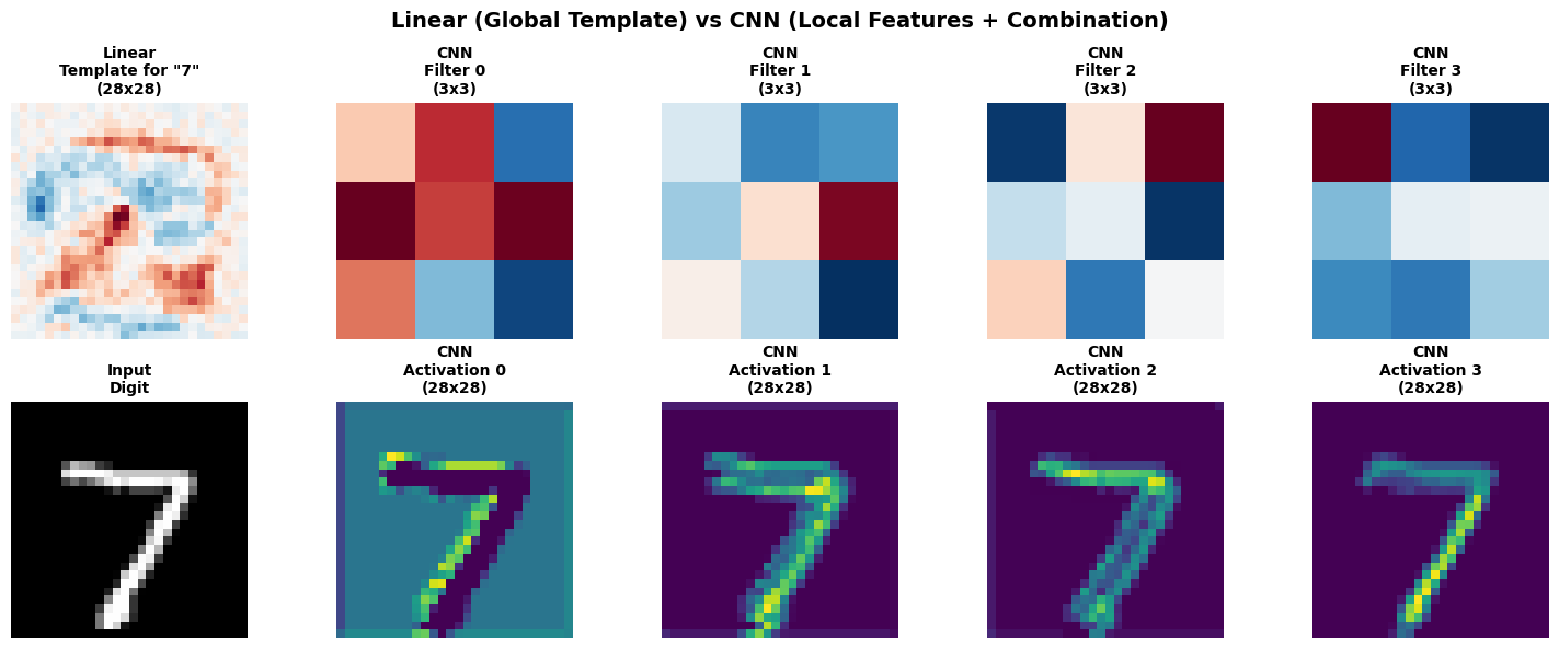
Key Differences
Linear Model:
- Learns ONE global template per digit (28×28 weight matrix)
- Classification: $y = \text{argmax}(W \cdot x)$ where $W \in \mathbb{R}^{10 \times 784}$
- Position-dependent: pixel at (i,j) has its own unique weight
- No feature reuse: each spatial location learned independently
- Cannot handle translation or rotation well
- Parameters: 7,850 (784 × 10 + 10 biases)
CNN:
- Learns MANY local feature detectors (3×3 filters)
- Each filter slides across entire image (translation invariance)
- Weight sharing: same 3×3 kernel applied at every position
- Hierarchical composition: edges → shapes → objects
- Spatial downsampling through pooling (reduces dimensionality)
- Parameters: ~207k total, but many shared across positions
Why CNN generalizes better despite more parameters:
- Inductive bias: Assumes spatial locality and translation invariance (true for images)
- Weight sharing: 3×3 filter has 9 weights, but applies to all 28×28=784 positions
- Compositionality: Builds complex features from simple ones (better sample efficiency)
Parameter count comparison:
- Linear: Every pixel gets its own weight → 784 × 10 = 7,840 parameters
- CNN conv1: 16 filters × (1 channel × 3 × 3) = 144 parameters (shared across 784 positions)
- Effective capacity is different from raw parameter count!
Summary: Why Convolutional Neural Networks Work
Mathematical Foundation
Convolution operation: \(F[i, j] = \sum_{m,n} I[i+m, j+n] \cdot K[m, n]\)
Key properties:
- Translation equivariance: Shifting input shifts output by same amount
- Local connectivity: Each output depends only on local input region
- Weight sharing: Same kernel applied everywhere
Architectural Principles
Hierarchy:
- Layer 1: Low-level features (edges, gradients)
- Layer 2: Mid-level features (curves, junctions)
- Deeper layers: High-level features (object parts)
- FC layers: Combination for classification
Dimensionality reduction:
- Convolution: Maintains or reduces spatial size
- Pooling: Aggressive downsampling (28×28 → 14×14 → 7×7)
- Final: Flatten to vector for classification
Efficiency through sharing:
- Same filter detects same feature everywhere
- Reduces parameters dramatically
- Enables learning from limited data
When to Use CNNs
CNNs excel when data has:
- Grid structure (images, spectrograms, time-series with channels)
- Spatial/temporal locality (nearby elements are related)
- Translation invariance (object identity independent of position)
- Compositional structure (complex features built from simple ones)
Extensions
Modern CNN architectures build on these principles:
- ResNet: Skip connections for very deep networks
- Inception: Multiple filter sizes in parallel
- DenseNet: Dense connections between layers
- U-Net: Encoder-decoder for segmentation
But the core idea remains: local features + weight sharing + hierarchical composition.