Matrices and Matrix Operations
![]()
Based on CS229 Linear Algebra Review - Section 2
Matrices are fundamental to machine learning. They represent datasets, transformations, and relationships between variables. In this notebook, we’ll explore matrix operations and their Python implementations.
import numpy as np
import matplotlib.pyplot as plt
import seaborn as sns
from mpl_toolkits.mplot3d import Axes3D

plt.style.use('seaborn-v0_8')
np.random.seed(42)
1. What is a Matrix?
Mathematical Definition
A matrix $\mathbf{A} \in \mathbb{R}^{m \times n}$ is a rectangular array of real numbers with $m$ rows and $n$ columns:
\[\mathbf{A} = \begin{bmatrix} a_{11} & a_{12} & \cdots & a_{1n} \\ a_{21} & a_{22} & \cdots & a_{2n} \\ \vdots & \vdots & \ddots & \vdots \\ a_{m1} & a_{m2} & \cdots & a_{mn} \end{bmatrix}\]In Machine Learning
- Data matrix: Each row is a sample, each column is a feature
- Transformation: Linear mappings between vector spaces
- Parameters: Model weights and coefficients
# Creating matrices in NumPy

# Method 1: From a list of lists
A = np.array([[1, 2, 3],
              [4, 5, 6]])
print(f"Matrix A:")
print(A)
print(f"Shape: {A.shape} (2 rows, 3 columns)")
print(f"Size: {A.size} elements")

# Method 2: Using NumPy functions
B = np.zeros((3, 3))  # 3x3 matrix of zeros
C = np.ones((2, 4))   # 2x4 matrix of ones
D = np.eye(3)         # 3x3 identity matrix
E = np.random.rand(2, 3)  # 2x3 random matrix

print(f"\nZeros matrix B:")
print(B)
print(f"\nOnes matrix C:")
print(C)
print(f"\nIdentity matrix D:")
print(D)
print(f"\nRandom matrix E:")
print(E)
Matrix A:
[[1 2 3]
 [4 5 6]]
Shape: (2, 3) (2 rows, 3 columns)
Size: 6 elements

Zeros matrix B:
[[0. 0. 0.]
 [0. 0. 0.]
 [0. 0. 0.]]

Ones matrix C:
[[1. 1. 1. 1.]
 [1. 1. 1. 1.]]

Identity matrix D:
[[1. 0. 0.]
 [0. 1. 0.]
 [0. 0. 1.]]

Random matrix E:
[[0.37454012 0.95071431 0.73199394]
 [0.59865848 0.15601864 0.15599452]]
2. Matrix Indexing and Slicing
Accessing Elements
- $a_{ij}$ is the element in row $i$, column $j$ (1-indexed in math, 0-indexed in Python)
- Rows and columns can be extracted as vectors
# Matrix indexing and slicing
M = np.array([[1, 2, 3, 4],
              [5, 6, 7, 8],
              [9, 10, 11, 12]])

print(f"Matrix M:")
print(M)
print()

# Access single element
print(f"Element at position (0,2): {M[0, 2]}")
print(f"Element at position (2,1): {M[2, 1]}")

# Access entire rows
print(f"\nFirst row: {M[0, :]}")
print(f"Second row: {M[1, :]}")

# Access entire columns
print(f"\nFirst column: {M[:, 0]}")
print(f"Third column: {M[:, 2]}")

# Submatrices
print(f"\nTop-left 2x2 submatrix:")
print(M[0:2, 0:2])

print(f"\nLast two rows, last two columns:")
print(M[1:, 2:])
Matrix M:
[[ 1  2  3  4]
 [ 5  6  7  8]
 [ 9 10 11 12]]

Element at position (0,2): 3
Element at position (2,1): 10

First row: [1 2 3 4]
Second row: [5 6 7 8]

First column: [1 5 9]
Third column: [ 3  7 11]

Top-left 2x2 submatrix:
[[1 2]
 [5 6]]

Last two rows, last two columns:
[[ 7  8]
 [11 12]]
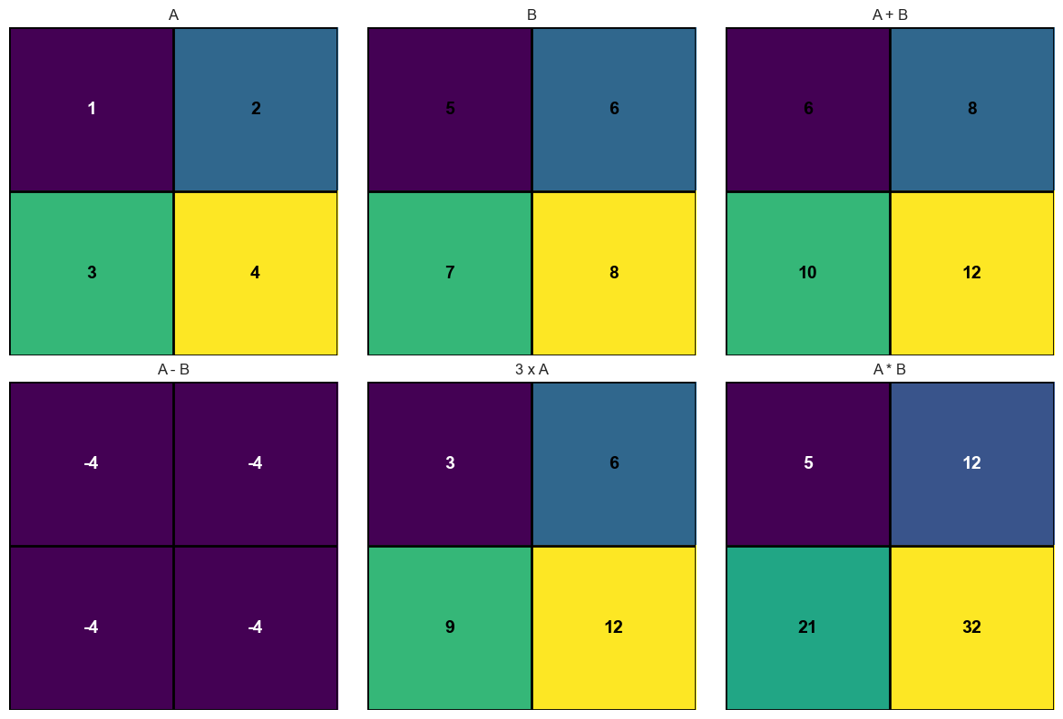
3. Matrix Addition and Scalar Multiplication
Mathematical Definition
For matrices $\mathbf{A}, \mathbf{B} \in \mathbb{R}^{m \times n}$:
Addition: $(\mathbf{A} + \mathbf{B}){ij} = a{ij} + b_{ij}$
Scalar multiplication: $(\alpha \mathbf{A}){ij} = \alpha a{ij}$
Note: Matrices must have the same dimensions for addition.
# Matrix addition and scalar multiplication
A = np.array([[1, 2],
              [3, 4]])
B = np.array([[5, 6],
              [7, 8]])

print(f"Matrix A:")
print(A)
print(f"\nMatrix B:")
print(B)

# Matrix addition
C = A + B
print(f"\nA + B:")
print(C)

# Matrix subtraction
D = A - B
print(f"\nA - B:")
print(D)

# Scalar multiplication
E = 3 * A
print(f"\n3 * A:")
print(E)

# Element-wise operations
F = A * B  # Element-wise multiplication (Hadamard product)
print(f"\nA * B (element-wise multiplication):")
print(F)

# Visualize matrix operations
fig, axes = plt.subplots(2, 3, figsize=(12, 8))
matrices = [A, B, C, D, E, F]
titles = ['A', 'B', 'A + B', 'A - B', '3 x A', 'A * B']

for i, (mat, title) in enumerate(zip(matrices, titles)):
    row, col = i // 3, i % 3
    im = axes[row, col].imshow(mat, cmap='viridis', aspect='equal')
    axes[row, col].set_title(title)

    # Add text annotations
    for r in range(mat.shape[0]):
        for c in range(mat.shape[1]):
            axes[row, col].text(c, r, f'{mat[r,c]:.0f}',
                               ha='center', va='center',
                               color='white' if mat[r,c] < mat.max()/2 else 'black',
                               fontsize=14, fontweight='bold')

    # Add grid lines with black borders
    axes[row, col].set_xticks(np.arange(-0.5, mat.shape[1], 1), minor=True)
    axes[row, col].set_yticks(np.arange(-0.5, mat.shape[0], 1), minor=True)
    axes[row, col].grid(which='minor', color='black', linestyle='-', linewidth=2)
    axes[row, col].set_xticks([])
    axes[row, col].set_yticks([])

plt.tight_layout()
plt.show()
Matrix A:
[[1 2]
 [3 4]]

Matrix B:
[[5 6]
 [7 8]]

A + B:
[[ 6  8]
 [10 12]]

A - B:
[[-4 -4]
 [-4 -4]]

3 * A:
[[ 3  6]
 [ 9 12]]

A * B (element-wise multiplication):
[[ 5 12]
 [21 32]]
4. Matrix Multiplication
Mathematical Definition
For $\mathbf{A} \in \mathbb{R}^{m \times n}$ and $\mathbf{B} \in \mathbb{R}^{n \times p}$:
\[(\mathbf{AB})_{ij} = \sum_{k=1}^n a_{ik} b_{kj}\]Key requirements:
- Number of columns in $\mathbf{A}$ must equal number of rows in $\mathbf{B}$
- Result is $m \times p$ matrix
Geometric Interpretation
Matrix multiplication represents composition of linear transformations.
# Matrix multiplication
A = np.array([[1, 2, 3],
              [4, 5, 6]])
B = np.array([[7, 8],
              [9, 10],
              [11, 12]])

print(f"Matrix A (2x3):")
print(A)
print(f"\nMatrix B (3x2):")
print(B)

# Matrix multiplication using @
C = A @ B
print(f"\nA @ B (2x2):")
print(C)

# Alternative: using np.dot
C_alt = np.dot(A, B)
print(f"\nUsing np.dot (same result):")
print(C_alt)

# Manual calculation for verification
print(f"\nManual calculation:")
print(f"C[0,0] = A[0,:] · B[:,0] = {A[0,:]} · {B[:,0]} = {np.dot(A[0,:], B[:,0])}")
print(f"C[0,1] = A[0,:] · B[:,1] = {A[0,:]} · {B[:,1]} = {np.dot(A[0,:], B[:,1])}")
print(f"C[1,0] = A[1,:] · B[:,0] = {A[1,:]} · {B[:,0]} = {np.dot(A[1,:], B[:,0])}")
print(f"C[1,1] = A[1,:] · B[:,1] = {A[1,:]} · {B[:,1]} = {np.dot(A[1,:], B[:,1])}")

# Dimension compatibility check
print(f"\nDimension compatibility:")
print(f"A.shape = {A.shape}, B.shape = {B.shape}")
print(f"A has {A.shape[1]} columns, B has {B.shape[0]} rows")
print(f"Since {A.shape[1]} == {B.shape[0]}, multiplication is valid")
print(f"Result shape: ({A.shape[0]}, {B.shape[1]}) = {C.shape}")
Matrix A (2x3):
[[1 2 3]
 [4 5 6]]

Matrix B (3x2):
[[ 7  8]
 [ 9 10]
 [11 12]]

A @ B (2x2):
[[ 58  64]
 [139 154]]

Using np.dot (same result):
[[ 58  64]
 [139 154]]

Manual calculation:
C[0,0] = A[0,:] · B[:,0] = [1 2 3] · [ 7  9 11] = 58
C[0,1] = A[0,:] · B[:,1] = [1 2 3] · [ 8 10 12] = 64
C[1,0] = A[1,:] · B[:,0] = [4 5 6] · [ 7  9 11] = 139
C[1,1] = A[1,:] · B[:,1] = [4 5 6] · [ 8 10 12] = 154

Dimension compatibility:
A.shape = (2, 3), B.shape = (3, 2)
A has 3 columns, B has 3 rows
Since 3 == 3, multiplication is valid
Result shape: (2, 2) = (2, 2)
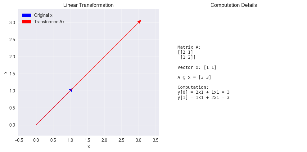
5. Matrix-Vector Multiplication
Mathematical Definition
For $\mathbf{A} \in \mathbb{R}^{m \times n}$ and $\mathbf{x} \in \mathbb{R}^n$:
\[\mathbf{Ax} = \begin{bmatrix} \mathbf{a}_1^T \mathbf{x} \\ \mathbf{a}_2^T \mathbf{x} \\ \vdots \\ \mathbf{a}_m^T \mathbf{x} \end{bmatrix}\]where $\mathbf{a}_i^T$ is the $i$-th row of $\mathbf{A}$.
In Machine Learning
This is fundamental for:
- Linear regression: $\hat{y} = \mathbf{Ax}$
- Neural networks: forward propagation
- Feature transformations
# Matrix-vector multiplication
A = np.array([[1, 2, 3],
              [4, 5, 6],
              [7, 8, 9]])
x = np.array([1, 2, 1])

print(f"Matrix A:")
print(A)
print(f"\nVector x: {x}")

# Matrix-vector multiplication
y = A @ x
print(f"\nA @ x = {y}")

# Show row-wise computation
print(f"\nRow-wise computation:")
for i in range(A.shape[0]):
    row_product = np.dot(A[i, :], x)
    print(f"Row {i}: {A[i, :]} · {x} = {row_product}")

# Visualize as linear transformation
# Let's use a 2D example for better visualization
A_2d = np.array([[2, 1],
                 [1, 2]])
x_2d = np.array([1, 1])
y_2d = A_2d @ x_2d

plt.figure(figsize=(10, 5))

# Plot original and transformed vectors
plt.subplot(1, 2, 1)
plt.arrow(0, 0, x_2d[0], x_2d[1], head_width=0.1, head_length=0.1,
          fc='blue', ec='blue', label='Original x')
plt.arrow(0, 0, y_2d[0], y_2d[1], head_width=0.1, head_length=0.1,
          fc='red', ec='red', label='Transformed Ax')
plt.grid(True, alpha=0.3)
plt.axis('equal')
plt.legend()
plt.title('Linear Transformation')
plt.xlabel('x')
plt.ylabel('y')

# Show the computation
plt.subplot(1, 2, 2)
computation_text = f"""Matrix A:
{A_2d}

Vector x: {x_2d}

A @ x = {y_2d}

Computation:
y[0] = {A_2d[0,0]}x{x_2d[0]} + {A_2d[0,1]}x{x_2d[1]} = {y_2d[0]}
y[1] = {A_2d[1,0]}x{x_2d[0]} + {A_2d[1,1]}x{x_2d[1]} = {y_2d[1]}"""
plt.text(0.1, 0.5, computation_text, transform=plt.gca().transAxes,
         fontsize=10, verticalalignment='center', fontfamily='monospace')
plt.axis('off')
plt.title('Computation Details')

plt.tight_layout()
plt.show()
Matrix A:
[[1 2 3]
 [4 5 6]
 [7 8 9]]

Vector x: [1 2 1]

A @ x = [ 8 20 32]

Row-wise computation:
Row 0: [1 2 3] · [1 2 1] = 8
Row 1: [4 5 6] · [1 2 1] = 20
Row 2: [7 8 9] · [1 2 1] = 32
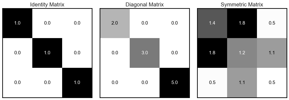
6. Special Matrices
Identity Matrix
The identity matrix $\mathbf{I} \in \mathbb{R}^{n \times n}$ has 1s on the diagonal and 0s elsewhere: \(\mathbf{I} = \begin{bmatrix} 1 & 0 & \cdots & 0 \\ 0 & 1 & \cdots & 0 \\ \vdots & \vdots & \ddots & \vdots \\ 0 & 0 & \cdots & 1 \end{bmatrix}\)
Property: $\mathbf{AI} = \mathbf{IA} = \mathbf{A}$ for any compatible matrix $\mathbf{A}$.
Diagonal Matrix
A matrix with non-zero elements only on the diagonal.
Symmetric Matrix
A matrix where $\mathbf{A} = \mathbf{A}^T$ (i.e., $a_{ij} = a_{ji}$).
# Special matrices
print("Special Matrices:")
print("=" * 30)

# Identity matrix
I = np.eye(3)
print(f"3x3 Identity matrix:")
print(I)

# Test identity property
A = np.random.randint(1, 10, (3, 3))
AI = A @ I
IA = I @ A
print(f"\nOriginal matrix A:")
print(A)
print(f"\nA @ I:")
print(AI)
print(f"\nI @ A:")
print(IA)
print(f"\nAre they equal? {np.allclose(A, AI) and np.allclose(A, IA)}")

# Diagonal matrix
diagonal_values = [2, 3, 5]
D = np.diag(diagonal_values)
print(f"\nDiagonal matrix with values {diagonal_values}:")
print(D)

# Symmetric matrix
# Create a symmetric matrix
B = np.random.rand(3, 3)
S = B + B.T  # Adding a matrix to its transpose makes it symmetric
print(f"\nSymmetric matrix S:")
print(S)
print(f"\nS transpose:")
print(S.T)
print(f"\nIs S symmetric? {np.allclose(S, S.T)}")
Special Matrices:
==============================
3x3 Identity matrix:
[[1. 0. 0.]
 [0. 1. 0.]
 [0. 0. 1.]]

Original matrix A:
[[2 4 5]
 [8 7 2]
 [5 4 4]]

A @ I:
[[2. 4. 5.]
 [8. 7. 2.]
 [5. 4. 4.]]

I @ A:
[[2. 4. 5.]
 [8. 7. 2.]
 [5. 4. 4.]]

Are they equal? True

Diagonal matrix with values [2, 3, 5]:
[[2 0 0]
 [0 3 0]
 [0 0 5]]

Symmetric matrix S:
[[1.40991766 1.7579063  0.50704232]
 [1.7579063  1.18635383 1.09057809]
 [0.50704232 1.09057809 0.4817118 ]]

S transpose:
[[1.40991766 1.7579063  0.50704232]
 [1.7579063  1.18635383 1.09057809]
 [0.50704232 1.09057809 0.4817118 ]]

Is S symmetric? True
# Visualize these matrices
fig, axes = plt.subplots(1, 3, figsize=(12, 4))
matrices = [I, D, S]
titles = ['Identity Matrix', 'Diagonal Matrix', 'Symmetric Matrix']

for i, (mat, title) in enumerate(zip(matrices, titles)):
    im = axes[i].imshow(mat, cmap='Greys', aspect='equal')
    axes[i].set_title(title, fontsize=16)

    # Add text annotations
    for r in range(mat.shape[0]):
        for c in range(mat.shape[1]):
            # Use white text on dark background, black text on light background
            text_color = 'white' if mat[r,c] > (mat.min() + mat.max()) / 2 else 'black'
            axes[i].text(c, r, f'{mat[r,c]:.1f}',
                        ha='center', va='center', fontsize=14,
                        color=text_color)

    # Add border and set white background
    axes[i].set_xticks([])
    axes[i].set_yticks([])
    axes[i].set_facecolor('white')
    for spine in axes[i].spines.values():
        spine.set_edgecolor('black')
        spine.set_linewidth(2)

plt.tight_layout()
plt.show()
7. Matrix Transpose
Mathematical Definition
The transpose of matrix $\mathbf{A} \in \mathbb{R}^{m \times n}$ is $\mathbf{A}^T \in \mathbb{R}^{n \times m}$ where: \((\mathbf{A}^T)_{ij} = a_{ji}\)
Properties
- $(\mathbf{A}^T)^T = \mathbf{A}$
- $(\mathbf{A} + \mathbf{B})^T = \mathbf{A}^T + \mathbf{B}^T$
- $(\mathbf{AB})^T = \mathbf{B}^T\mathbf{A}^T$
# Matrix transpose
A = np.array([[1, 2, 3],
              [4, 5, 6]])

print(f"Original matrix A (2x3):")
print(A)

# Transpose
A_T = A.T
print(f"\nTranspose A^T (3x2):")
print(A_T)

# Alternative method
A_T_alt = np.transpose(A)
print(f"\nUsing np.transpose (same result):")
print(A_T_alt)

# Verify properties
print(f"\nVerifying properties:")
print(f"(A^T)^T == A? {np.array_equal(A_T.T, A)}")

# For matrix multiplication property
B = np.array([[1, 2],
              [3, 4],
              [5, 6]])
AB = A @ B
AB_T = AB.T
BT_AT = B.T @ A.T

print(f"\nMatrix B (3x2):")
print(B)
print(f"\nAB (2x2):")
print(AB)
print(f"\n(AB)^T:")
print(AB_T)
print(f"\nB^T @ A^T:")
print(BT_AT)
print(f"\n(AB)^T == B^T A^T? {np.allclose(AB_T, BT_AT)}")
Original matrix A (2x3):
[[1 2 3]
 [4 5 6]]

Transpose A^T (3x2):
[[1 4]
 [2 5]
 [3 6]]

Using np.transpose (same result):
[[1 4]
 [2 5]
 [3 6]]

Verifying properties:
(A^T)^T == A? True

Matrix B (3x2):
[[1 2]
 [3 4]
 [5 6]]

AB (2x2):
[[22 28]
 [49 64]]

(AB)^T:
[[22 49]
 [28 64]]

B^T @ A^T:
[[22 49]
 [28 64]]

(AB)^T == B^T A^T? True
8. Practice Exercises
Work through these exercises to solidify your understanding:
# Practice Exercise: Matrix Operations
print("Practice Exercises:")
print("=" * 30)

# Create random matrices for practice
np.random.seed(123)  # For reproducible results
A = np.random.randint(1, 6, (3, 3))
B = np.random.randint(1, 6, (3, 3))
x = np.random.randint(1, 6, 3)

print(f"Matrix A:")
print(A)
print(f"\nMatrix B:")
print(B)
print(f"\nVector x: {x}")

# Exercise 1: Basic operations
print(f"\nExercise 1: Basic Operations")
print(f"A + B =")
print(A + B)

print(f"\nA - B =")
print(A - B)

print(f"\n2 * A =")
print(2 * A)

# Exercise 2: Matrix multiplication
print(f"\nExercise 2: Matrix Multiplication")
print(f"A @ B =")
print(A @ B)

print(f"\nB @ A =")
print(B @ A)
print(f"\nNote: A @ B ≠ B @ A (matrix multiplication is not commutative!)")

# Exercise 3: Matrix-vector multiplication
print(f"\nExercise 3: Matrix-Vector Multiplication")
y = A @ x
print(f"A @ x = {y}")

# Exercise 4: Transpose properties
print(f"\nExercise 4: Transpose Properties")
AT = A.T
BT = B.T
AB = A @ B
AB_T = AB.T
BT_AT = BT @ AT

print(f"(A @ B)^T =")
print(AB_T)
print(f"\nB^T @ A^T =")
print(BT_AT)
print(f"\nAre they equal? {np.allclose(AB_T, BT_AT)}")

# Exercise 5: Check if matrix is symmetric
print(f"\nExercise 5: Symmetry Check")
S = A @ A.T  # This creates a symmetric matrix
print(f"S = A @ A^T =")
print(S)
print(f"\nIs S symmetric? {np.allclose(S, S.T)}")
print(f"\nS^T =")
print(S.T)
Practice Exercises:
==============================
Matrix A:
[[3 5 3]
 [2 4 3]
 [4 2 2]]

Matrix B:
[[1 2 2]
 [1 1 2]
 [4 5 1]]

Vector x: [1 5 2]

Exercise 1: Basic Operations
A + B =
[[4 7 5]
 [3 5 5]
 [8 7 3]]

A - B =
[[ 2  3  1]
 [ 1  3  1]
 [ 0 -3  1]]

2 * A =
[[ 6 10  6]
 [ 4  8  6]
 [ 8  4  4]]

Exercise 2: Matrix Multiplication
A @ B =
[[20 26 19]
 [18 23 15]
 [14 20 14]]

B @ A =
[[15 17 13]
 [13 13 10]
 [26 42 29]]

Note: A @ B ≠ B @ A (matrix multiplication is not commutative!)

Exercise 3: Matrix-Vector Multiplication
A @ x = [34 28 18]

Exercise 4: Transpose Properties
(A @ B)^T =
[[20 18 14]
 [26 23 20]
 [19 15 14]]

B^T @ A^T =
[[20 18 14]
 [26 23 20]
 [19 15 14]]

Are they equal? True

Exercise 5: Symmetry Check
S = A @ A^T =
[[43 35 28]
 [35 29 22]
 [28 22 24]]

Is S symmetric? True

S^T =
[[43 35 28]
 [35 29 22]
 [28 22 24]]
Key Takeaways
- Matrices represent data: In ML, matrices store datasets and transformations
- Matrix multiplication is fundamental: Core operation in linear algebra and ML
- Dimensions must match: Always check compatibility for operations
- Order matters: Matrix multiplication is not commutative ($\mathbf{AB} \neq \mathbf{BA}$)
- Transpose has important properties: Especially for matrix multiplication
- Special matrices have special roles: Identity, diagonal, and symmetric matrices
Next Steps
In the next notebook, we’ll explore matrix inversion, determinants, and eigenvalues - concepts that are crucial for understanding how machine learning algorithms work under the hood.