Vectors and Basic Operations
![]()
Based on CS229 Linear Algebra Review - Section 1
In this notebook, we’ll explore the fundamental building blocks of linear algebra that are essential for machine learning: vectors and their operations.
import numpy as np
import matplotlib.pyplot as plt
import seaborn as sns

# Set up plotting
plt.style.use('seaborn-v0_8')
np.random.seed(42)
1. What is a Vector?
Mathematical Definition
A vector $\mathbf{x} \in \mathbb{R}^n$ is an ordered collection of $n$ real numbers. We can write it as:
\[\mathbf{x} = \begin{bmatrix} x_1 \\ x_2 \\ \vdots \\ x_n \end{bmatrix}\]Geometric Interpretation
A vector represents:
- A point in n-dimensional space
- A direction and magnitude from the origin
- A displacement or movement
# Create vectors in Python using NumPy
# A 3-dimensional vector
x = np.array([2, 3, 1])
print(f"Vector x: {x}")
print(f"Shape: {x.shape}")
print(f"Dimension: {len(x)}")

# Another vector
y = np.array([1, -2, 4])
print(f"\nVector y: {y}")
Vector x: [2 3 1]
Shape: (3,)
Dimension: 3

Vector y: [ 1 -2  4]
2. Vector Addition
Mathematical Definition
For vectors $\mathbf{x}, \mathbf{y} \in \mathbb{R}^n$:
\[\mathbf{x} + \mathbf{y} = \begin{bmatrix} x_1 + y_1 \\ x_2 + y_2 \\ \vdots \\ x_n + y_n \end{bmatrix}\]Geometric Interpretation
Vector addition follows the “tip-to-tail” rule or parallelogram rule.
# Vector addition in NumPy
vector_sum = x + y
print(f"x + y = {vector_sum}")

# Let's visualize 2D vector addition
# Create 2D vectors for visualization
a = np.array([3, 2])
b = np.array([1, 3])
c = a + b

plt.figure(figsize=(8, 6))
# Plot vectors from origin
plt.arrow(0, 0, a[0], a[1], head_width=0.2, head_length=0.2, fc='blue', ec='blue', label='Vector a')
plt.arrow(0, 0, b[0], b[1], head_width=0.2, head_length=0.2, fc='red', ec='red', label='Vector b')
plt.arrow(0, 0, c[0], c[1], head_width=0.2, head_length=0.2, fc='green', ec='green', label='a + b')

# Show tip-to-tail addition
plt.arrow(a[0], a[1], b[0], b[1], head_width=0.1, head_length=0.1, fc='red', ec='red', alpha=0.5, linestyle='--')

plt.grid(True, alpha=0.3)
plt.axis('equal')
plt.legend()
plt.title('Vector Addition: Tip-to-Tail Rule')
plt.xlabel('x')
plt.ylabel('y')
plt.show()

print(f"a = {a}")
print(f"b = {b}")
print(f"a + b = {c}")
x + y = [3 1 5]
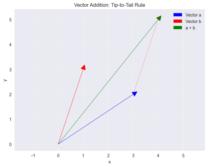
a = [3 2]
b = [1 3]
a + b = [4 5]
3. Scalar Multiplication
Mathematical Definition
For a scalar $\alpha \in \mathbb{R}$ and vector $\mathbf{x} \in \mathbb{R}^n$:
\[\alpha \mathbf{x} = \begin{bmatrix} \alpha x_1 \\ \alpha x_2 \\ \vdots \\ \alpha x_n \end{bmatrix}\]Geometric Interpretation
- If $\alpha > 1$: stretches the vector
- If $0 < \alpha < 1$: shrinks the vector
- If $\alpha < 0$: flips direction and scales magnitude
# Scalar multiplication
v = np.array([2, 1])
scalars = [0.5, 1, 2, -1]

plt.figure(figsize=(10, 6))
colors = ['orange', 'blue', 'green', 'red']

for i, alpha in enumerate(scalars):
    scaled_v = alpha * v
    plt.arrow(0, 0, scaled_v[0], scaled_v[1],
              head_width=0.2, head_length=0.2,
              fc=colors[i], ec=colors[i],
              label=f'{alpha} x v = {scaled_v}')

plt.grid(True, alpha=0.3)
plt.axis('equal')
plt.legend()
plt.title('Scalar Multiplication of Vectors')
plt.xlabel('x')
plt.ylabel('y')
plt.xlim(-3, 5)
plt.ylim(-3, 3)
plt.show()

# Show the calculations
print(f"Original vector v: {v}")
for alpha in scalars:
    result = alpha * v
    print(f"{alpha} x v = {result}")
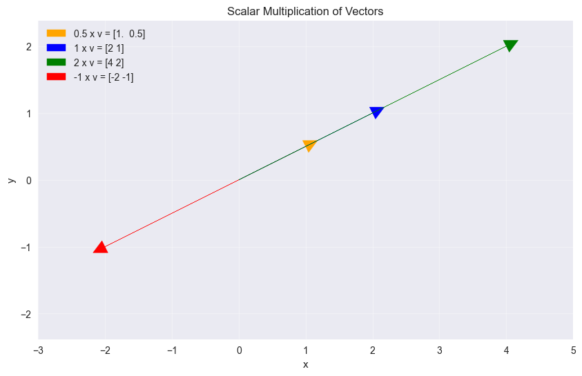
Original vector v: [2 1]
0.5 x v = [1.  0.5]
1 x v = [2 1]
2 x v = [4 2]
-1 x v = [-2 -1]
4. Vector Norms (Length/Magnitude)
Mathematical Definition
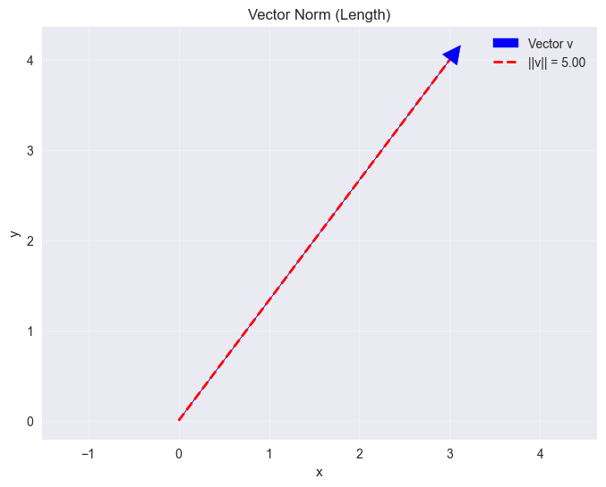
The Euclidean norm (or L2 norm) of a vector $\mathbf{x} \in \mathbb{R}^n$ is:
\[\|\mathbf{x}\|_2 = \sqrt{x_1^2 + x_2^2 + \cdots + x_n^2} = \sqrt{\mathbf{x}^T\mathbf{x}}\]This measures the “length” or “magnitude” of the vector.
# Calculate vector norms
v = np.array([3, 4])

# Method 1: Using NumPy's norm function
norm_v = np.linalg.norm(v)
print(f"Vector v: {v}")
print(f"||v||_2 using np.linalg.norm: {norm_v}")

# Method 2: Manual calculation
norm_manual = np.sqrt(np.sum(v**2))
print(f"||v||_2 manual calculation: {norm_manual}")

# Method 3: Using dot product
norm_dot = np.sqrt(np.dot(v, v))
print(f"||v||_2 using dot product: {norm_dot}")

# Visualize the norm
plt.figure(figsize=(8, 6))
plt.arrow(0, 0, v[0], v[1], head_width=0.2, head_length=0.2, fc='blue', ec='blue', label='Vector v')
plt.plot([0, v[0]], [0, v[1]], 'r--', linewidth=2, label=f'||v|| = {norm_v:.2f}')

plt.grid(True, alpha=0.3)
plt.axis('equal')
plt.legend()
plt.title('Vector Norm (Length)')
plt.xlabel('x')
plt.ylabel('y')
plt.show()

# Example with 3D vector
v3d = np.array([1, 2, 2])
print(f"\n3D vector: {v3d}")
print(f"||v||_2 = {np.linalg.norm(v3d):.3f}")
Vector v: [3 4]
||v||_2 using np.linalg.norm: 5.0
||v||_2 manual calculation: 5.0
||v||_2 using dot product: 5.0
3D vector: [1 2 2]
||v||_2 = 3.000
5. Unit Vectors and Normalization
Mathematical Definition
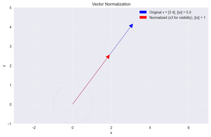
A unit vector has norm equal to 1. We can normalize any non-zero vector $\mathbf{x}$ to get a unit vector:
\[\hat{\mathbf{x}} = \frac{\mathbf{x}}{\|\mathbf{x}\|}\]This preserves the direction but sets the magnitude to 1.
# Vector normalization
v = np.array([3, 4, 0])
print(f"Original vector: {v}")
print(f"Original norm: {np.linalg.norm(v)}")

# Normalize the vector
v_normalized = v / np.linalg.norm(v)
print(f"\nNormalized vector: {v_normalized}")
print(f"Normalized norm: {np.linalg.norm(v_normalized)}")

# Alternative using sklearn's normalize
# But let's do it manually for educational purposes

# Visualize original vs normalized
plt.figure(figsize=(10, 6))

# Original vector (only first 2 components for visualization)
plt.arrow(0, 0, v[0], v[1], head_width=0.2, head_length=0.2,
          fc='blue', ec='blue', label=f'Original v = {v[:2]}, ||v|| = {np.linalg.norm(v):.1f}')

# Normalized vector (scaled up for visibility)
scale = 3  # Scale for visualization
v_norm_scaled = v_normalized[:2] * scale
plt.arrow(0, 0, v_norm_scaled[0], v_norm_scaled[1], head_width=0.2, head_length=0.2,
          fc='red', ec='red', label=f'Normalized (x{scale} for visibility), ||v|| = 1')

# Unit circle for reference
circle = plt.Circle((0, 0), 1, fill=False, color='gray', linestyle='--', alpha=0.5)
plt.gca().add_patch(circle)

plt.grid(True, alpha=0.3)
plt.axis('equal')
plt.legend()
plt.title('Vector Normalization')
plt.xlabel('x')
plt.ylabel('y')
plt.xlim(-1, 5)
plt.ylim(-1, 5)
plt.show()
Original vector: [3 4 0]
Original norm: 5.0

Normalized vector: [0.6 0.8 0. ]
Normalized norm: 1.0
6. Dot Product (Inner Product)
Mathematical Definition
For vectors $\mathbf{x}, \mathbf{y} \in \mathbb{R}^n$:
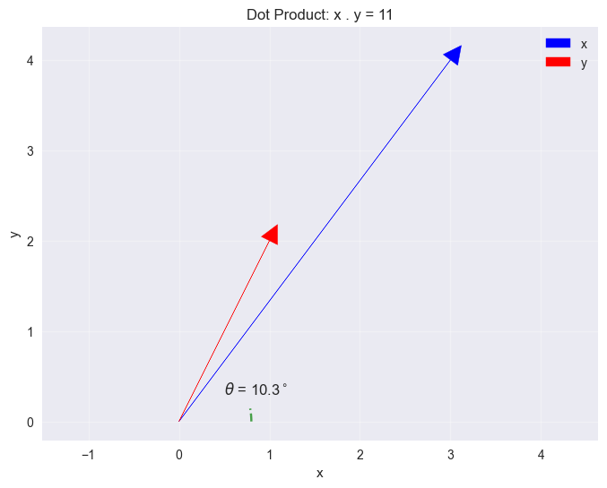
\[\mathbf{x} \cdot \mathbf{y} = \mathbf{x}^T\mathbf{y} = \sum_{i=1}^n x_i y_i = x_1 y_1 + x_2 y_2 + \cdots + x_n y_n\]Geometric Interpretation
\(\mathbf{x} \cdot \mathbf{y} = \|\mathbf{x}\| \|\mathbf{y}\| \cos(\theta)\)
where $\theta$ is the angle between the vectors.
# Dot product examples
x = np.array([3, 4])
y = np.array([1, 2])

# Calculate dot product
dot_product = np.dot(x, y)
print(f"x = {x}")
print(f"y = {y}")
print(f"x . y = {dot_product}")

# Manual calculation
dot_manual = x[0]*y[0] + x[1]*y[1]
print(f"Manual calculation: {x[0]}x{y[0]} + {x[1]}x{y[1]} = {dot_manual}")

# Calculate angle between vectors
cos_theta = dot_product / (np.linalg.norm(x) * np.linalg.norm(y))
theta_radians = np.arccos(cos_theta)
theta_degrees = np.degrees(theta_radians)

print(f"\nAngle between vectors: {theta_degrees:.1f} degrees")

# Visualize
plt.figure(figsize=(8, 6))
plt.arrow(0, 0, x[0], x[1], head_width=0.2, head_length=0.2, fc='blue', ec='blue', label='x')
plt.arrow(0, 0, y[0], y[1], head_width=0.2, head_length=0.2, fc='red', ec='red', label='y')

# Draw angle arc
angles = np.linspace(0, theta_radians, 50)
arc_radius = 0.8
arc_x = arc_radius * np.cos(angles)
arc_y = arc_radius * np.sin(angles)
plt.plot(arc_x, arc_y, 'g--', alpha=0.7)
plt.text(0.5, 0.3, f'$\\theta$ = {theta_degrees:.1f}$^\circ$', fontsize=12)

plt.grid(True, alpha=0.3)
plt.axis('equal')
plt.legend()
plt.title(f'Dot Product: x . y = {dot_product}')
plt.xlabel('x')
plt.ylabel('y')
plt.show()
x = [3 4]
y = [1 2]
x . y = 11
Manual calculation: 3x1 + 4x2 = 11

Angle between vectors: 10.3 degrees
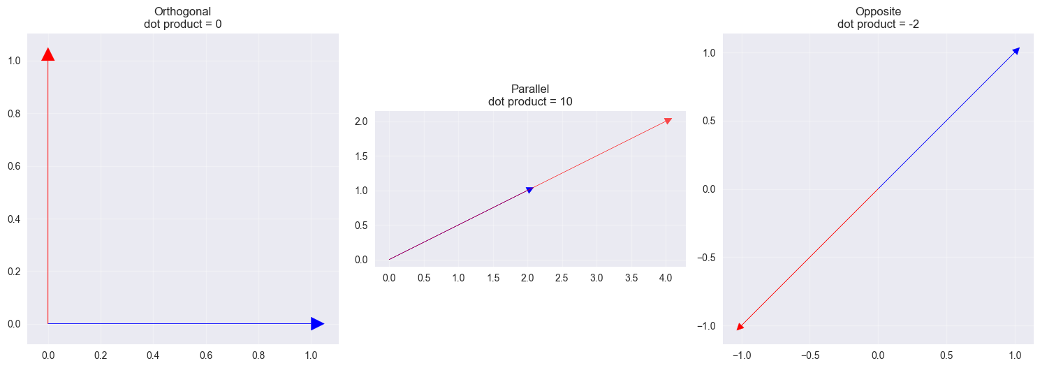
7. Special Cases of Dot Product
Orthogonal Vectors
When $\mathbf{x} \cdot \mathbf{y} = 0$, the vectors are orthogonal (perpendicular).
Parallel Vectors
When vectors point in the same direction, $\cos(\theta) = 1$, so $\mathbf{x} \cdot \mathbf{y} = |\mathbf{x}| |\mathbf{y}|$.
# Examples of special cases
print("Special Cases of Dot Product:")
print("=" * 40)

# Orthogonal vectors
v1 = np.array([1, 0])
v2 = np.array([0, 1])
dot1 = np.dot(v1, v2)
print(f"Orthogonal vectors: {v1} . {v2} = {dot1}")

# Parallel vectors (same direction)
v3 = np.array([2, 1])
v4 = np.array([4, 2])  # 2 * v3
dot2 = np.dot(v3, v4)
expected = np.linalg.norm(v3) * np.linalg.norm(v4)
print(f"Parallel vectors: {v3} . {v4} = {dot2}")
print(f"Expected (||v3|| x ||v4||): {expected:.3f}")

# Opposite direction
v5 = np.array([1, 1])
v6 = np.array([-1, -1])  # opposite direction
dot3 = np.dot(v5, v6)
expected_neg = -np.linalg.norm(v5) * np.linalg.norm(v6)
print(f"Opposite vectors: {v5} . {v6} = {dot3}")
print(f"Expected (-||v5|| x ||v6||): {expected_neg:.3f}")

# Visualize all cases
fig, axes = plt.subplots(1, 3, figsize=(15, 5))

# Orthogonal
axes[0].arrow(0, 0, v1[0], v1[1], head_width=0.05, head_length=0.05, fc='blue', ec='blue')
axes[0].arrow(0, 0, v2[0], v2[1], head_width=0.05, head_length=0.05, fc='red', ec='red')
axes[0].set_title(f'Orthogonal\ndot product = {dot1}')
axes[0].grid(True, alpha=0.3)
axes[0].set_aspect('equal')

# Parallel
axes[1].arrow(0, 0, v3[0], v3[1], head_width=0.1, head_length=0.1, fc='blue', ec='blue')
axes[1].arrow(0, 0, v4[0], v4[1], head_width=0.1, head_length=0.1, fc='red', ec='red', alpha=0.7)
axes[1].set_title(f'Parallel\ndot product = {dot2}')
axes[1].grid(True, alpha=0.3)
axes[1].set_aspect('equal')

# Opposite
axes[2].arrow(0, 0, v5[0], v5[1], head_width=0.05, head_length=0.05, fc='blue', ec='blue')
axes[2].arrow(0, 0, v6[0], v6[1], head_width=0.05, head_length=0.05, fc='red', ec='red')
axes[2].set_title(f'Opposite\ndot product = {dot3}')
axes[2].grid(True, alpha=0.3)
axes[2].set_aspect('equal')

plt.tight_layout()
plt.show()
Special Cases of Dot Product:
========================================
Orthogonal vectors: [1 0] . [0 1] = 0
Parallel vectors: [2 1] . [4 2] = 10
Expected (||v3|| x ||v4||): 10.000
Opposite vectors: [1 1] . [-1 -1] = -2
Expected (-||v5|| x ||v6||): -2.000
8. Practice Exercises
Try these exercises to test your understanding:
# Exercise 1: Create and manipulate vectors
print("Exercise 1: Vector Operations")
print("=" * 30)

# Create two random vectors
a = np.random.randint(-5, 6, 3)
b = np.random.randint(-5, 6, 3)

print(f"a = {a}")
print(f"b = {b}")

# TODO: Calculate the following (replace None with your code)
vector_sum = a + b  # a + b
vector_diff = a - b  # a - b
scalar_mult = 3 * a  # 3 * a
dot_prod = np.dot(a, b)  # a . b
norm_a = np.linalg.norm(a)  # ||a||
norm_b = np.linalg.norm(b)  # ||b||

print(f"\nResults:")
print(f"a + b = {vector_sum}")
print(f"a - b = {vector_diff}")
print(f"3 * a = {scalar_mult}")
print(f"a . b = {dot_prod}")
print(f"||a|| = {norm_a:.3f}")
print(f"||b|| = {norm_b:.3f}")

# Calculate angle between vectors
if norm_a > 0 and norm_b > 0:  # Avoid division by zero
    cos_angle = dot_prod / (norm_a * norm_b)
    angle_deg = np.degrees(np.arccos(np.clip(cos_angle, -1, 1)))
    print(f"Angle between a and b: {angle_deg:.1f} degrees")
Exercise 1: Vector Operations
==============================
a = [ 1 -2  5]
b = [ 2 -1  1]

Results:
a + b = [ 3 -3  6]
a - b = [-1 -1  4]
3 * a = [ 3 -6 15]
a . b = 9
||a|| = 5.477
||b|| = 2.449
Angle between a and b: 47.9 degrees
Key Takeaways
- Vectors are fundamental: They represent data points, features, and directions in ML
- NumPy makes it easy: Vector operations are simple and efficient
- Geometric intuition matters: Understanding vectors geometrically helps with ML concepts
- Dot products measure similarity: Fundamental for many ML algorithms
- Normalization is common: Unit vectors are frequently used in ML
Next Steps
In the next notebook, we’ll explore matrices and matrix operations, building on these vector concepts to understand higher-dimensional data and linear transformations.